3 http://0-2000webhosting.co.uk/choosedomain.asp. 4 http://0-2000webhosting.co.uk/comparison-web-hosting.htm. Input. Output. 0. 1. 2. 3. 4. 5. 1 3. 4 5. 0 3. 3.
AUTOMATYKA 2011 Tom 15 Zeszyt 3
Micha³ Sima*, Wojciech Bieniecki*, Szymon Grabowski*
Web Graph Visualizer 1. Introduction Web Graph is a directed, unlabeled graph G = (V, E), which represents connections between web documents on the Internet. It consists of two sets: V – vertices (nodes) for individual documents, and E – edges between nodes, i.e., the links between web documents. The com-plete Web Graph is a huge structure. As of October 2011, it is estimated (http:// www.worldwidewebsize.com/) that Google's index has about 40 billion web pages. In practice we are thus able to deal with relative small crawls, e.g., a single country domain. Visual representation of Web Graph allows to study the relationship between chosen sites more thoroughly. While knowing how to interpret obtained graphical representation, one is able to find not only web spam [1] or quality of links in a single website, but also examine, if investigated website is popular or positioned well enough in relation to any search engine algorithm, e.g. PageRank. Studying changes in Web Graph over time one can inspect how information about a particular site spreads on the web, witnessing not only its popularity, but also the regions of the web linked to it. Hence, the tools representing Web Graph may be helpful during positioning process as well as planning advertisement campaigns in the Internet. Not only web spam might be found this way, but also web communities or link farms. Finally, seeing the 2D graph structure may give ideas for efficient lossless compression algorithms of such graphs. For example, in [2] six types of blocks in a graph matrix have been described, including a singleton block, a horizontal block, a vertical block, an L-shaped block and a rectangular block (see Fig. 1). Visual inspection of large graphs may however let us broaden this collection of primitives. A Web Graph visualizer should allow for common operations on the graph, that is: visualize the adjacency matrix. This is an n×n matrix where n is the number of nodes. The entry aij contains the number of edges between node i and j (0 or 1 only; even if there are duplicated hyperlinks, we ignore them); show the direct neighbors (outgoing links) for a given web page; show the reverse neighbors (incoming links) for a given page. * Computer Engineering Department, Technical University of Lodz, Poland
259
260
Micha³ Sima, Wojciech Bieniecki, Szymon Grabowski
WebGraph Explorer is our application for Web Graph visualization. It allows to navigate freely over the adjacency matrix. In particular, the user can drag or shift the current graph view area and change the zoom scale (from node-to-pixel mapping up to fitting the whole matrix within a single rendering panel). The application is fully configurable (keyboard shortcuts, used colors etc.). The current view area can be copied or exported to an image file. WebGraph Explorer allows to work with several web graphs (crawls) simultaneously, shown on separate tabs. The current workspace (all open graphs and the program state) can be saved to a file. Hence, one can interrupt his work and easily return to it later. The program was written in C# 4.0, in Microsoft Visual Studio 2010 environment, and requires .NET 4.0. 0
1
0
2
3
4
1
1
1
5
6
7
1
1
1
1
1
1
1
1
1
1
1
1
8
9
1 2 3
1 1
4
1
5
1
1
6
1
7
1
8
1
9
1
1
1
1
1
1 1 1
Fig. 1. Exemplary adjacency matrix primitives, as defined in [2]
2. Input files for visualization We use two input files, both textual, one containing the structure of a graph and another with corresponding URLs. Only the first one is required as Web Graph might be rendered without information about the actual URLs. The first file stores adjacency lists for the successive nodes, each in a separate line. The adjacency lists store ascending IDs (integers) of all the outgoing links. This convention (often in binary form) is commonly used in the literature on Web Graph algorithms (see Fig. 2 with an example). Document #2 (http://0-2000webhosting.co.uk/business-web-hosting.htm) has 16 outgoing links, including one to document #1 (http://0-2000webhosting.co.uk/about-0-2000webhosting.htm). Please note, that the contents of the matrix depends on the ordering of the graph nodes, but the graphs induced by various orderings are of course isomorphic. The most commonly used form of storing Web crawls keeps the nodes sorted in their URL lexicographical order. In this case, the URLs belonging to one site are stored in successive lines and so is with the corresponding adjacency lists. This ordering is rather beneficial for the graph compression,
Web Graph Visualizer
261
as pages from the same site tend to have similar link patterns. Interestingly, also other compression-friendly node orderings were considered [3], but then the compression of the URLs themselves is hampered.
No. 0 1 2 3 4 No. 0 1 2 3 4
Beginning of the UK-2002 adjacency lists file 1 2 5 7 9 13 14 15 20 23 25 27 1888911 1 5 7 13 14 25 27 1 2 4 5 7 9 13 14 16 17 21 23 25 26 27 29 1 5 7 13 14 25 27 28 1 2 4 5 7 9 13 14 16 17 21 23 25 26 27 29 30 31 Beginning of the UK-2002 URL file http://0-2000webhosting.co.uk/ http://0-2000webhosting.co.uk/about-0-2000webhosting.htm http://0-2000webhosting.co.uk/business-web-hosting.htm http://0-2000webhosting.co.uk/choosedomain.asp http://0-2000webhosting.co.uk/comparison-web-hosting.htm Fig. 2. Adjacency lists and URL data from the beginning of UK-2002 [4]
3. The output WebGraph Explorer renders an image which represents the adjacency matrix of Web Graph. By default, nodes are represented by columns. Each web document has assigned a zero-based number corresponding to a column. The hyperlink between two documents is represented as a single dot (dark pixel) in the image, for example if document #4 contains a hyperlink to document #3, then the pixel in column 4, row 3 will be black (Fig. 3). Input
0 1 2 3 4 5
Output
13 45 03 3 0123
Fig. 3. A tiny graph and its visual representation. Each square is a single pixel
262
Micha³ Sima, Wojciech Bieniecki, Szymon Grabowski
In many cases we are interested in viewing a large part of the graph “on a single screen”. This implies representing many adjacent matrix cells (as squares) with individual pixels. In terms of the application functionality it means that that, after zooming out, one pixel on the screen represents a larger area of the original graph, and the rendered grayscale pixel is darker proportionally to the fraction of hyperlinks in the square it represents (Fig. 4 illustrates).
Fig. 4. Scaling of a graph
As web documents from the same site are kept in adjacent lines of the input file, we can easily investigate a single website with d documents by reducing the rendered matrix to the corresponding subset of d adjacent columns, or only to a respective d×d square, if only internal hyperlinks are within our interest.
4. User interface features In Figure 5 the main window of Web Graph Explorer is shown. The list of operations available from the main toolbar include: 1 – Add new graph to the current workspace, 2 – Save workspace to a file, 3 – Export current (or all) graph(s) to an image file, 4 – Copy current graph to Clipboard, 5 – Change rendering options, 6 – Customize colors, 7 – Change shortcuts, 8 – Enable tooltip for a hyperlink, 9 – Enable tooltip for blank space, 10 – Enable tooltip with total number of hyperlinks in a hover pixel, 11 – Show statistics of a graph, 12 – Show About box, 13 – Go to other area in the graph, 14–15 – Zoom in / out, 16–19 – Go left / right / up / down, 20 – Auto-reloading (if disabled, zooming will be done without re-rendering), 21 – Enable moving by the size of current image (like Page Down / Page Up), 22 – Enable skipping blank spaces while navigating (#21 will be also enabled), 23 – Force refresh of a graph (useful for instance if colors were change), 24 – Clear cache memory (in order to free some RAM), 25 – Manage bookmarks. Many graphs may be open at the same time, in tabbed pages. Current workspace (opened graphs and Notes) may be saved to a file and then will automatically be restored at
Web Graph Visualizer
263
the next program execution. Rendered graph can be exported to an image (JPEG, PNG, GIF, BMP) or copied to clipboard. When many graphs are open, the user may export all of them at once, with consecutive numbers being added at the beginning of a chosen filename.
Fig. 5. Main toolbar
In the Customize dialog window (Fig. 6) a user can change shortcuts bound to various actions.
Fig. 6. Dialog window with program custom options
264
Micha³ Sima, Wojciech Bieniecki, Szymon Grabowski
What is more, following rendering options can be modified at any time: Highlighting documents from the same website with alternating background colors (Fig. 7); using this feature requires the corresponding URL file. Use Threshold (Fig. 8). When it is enabled, the pixel on the result image will be marked as a hyperlink only if the percentage of hyperlinks in the respective area exceeds selected value. If disabled, the color intensity will represent the percentage of hyperlinks in a single pixel. Set the maximum number of lines stored in the buffer. By default, all lines which are used in the displayed image are buffered in order to speed up navigation. However, after zooming out a lot (for example, when 400×400 blocks per pixel are used) the buffer would need too much memory. Set the step, i.e., the distance (in pixels) by which the current location will be moved after an arrow click. The colors for different areas and objects can also be customized. They include the hyperlinks, empty spaces, border (out of the graph) area and odd/even websites (Fig. 7).
Fig. 7. Websites separation with odd and even background color
There are three main tab pages: Web Graphs, Web browser, Notes. The first one contains all opened graphs, the second one is a web browser (where one can see any website, not only those available in the Context Menu) and the last one is a simple notepad (useful for writing graph descriptions). All main features are available in the main menu (Fig. 9). Most of them are also available on the main toolbar (Fig. 5) and were already described. Current shortcuts are visible (next to the option): 1. jump to a corner of a graph, 2. show the center of a graph, 3. go in the chosen direction till the boundary of the graph. The user can also copy the list of URLs in the selected graph area or open the interesting page using a web browser widget.
Web Graph Visualizer
265
With a right-click on the graph, a user can open in the web browser one of the websites which are represented by a hovered pixel. All outgoing, incoming or both links (URLs), as well as the total number of hyperlinks in the pixel (its density) can be copied to the clipboard. The program provides a system of bookmarks (Fig. 10), to mark and then retrieve an interesting location in the graph. The status bar may optionally show the current location and other basic information.
Fig. 8. Zooming. Threshold example
Fig. 9. Main menu
266
Micha³ Sima, Wojciech Bieniecki, Szymon Grabowski
Fig. 10. Bookmark manager
In order to add a new graph (Fig. 11), the user must choose a single input file with Web Graph structure and can (additionally) choose the corresponding file with the URLs.
Fig. 11. Adding a new graph
It is possible to transpose a graph (as if the adjacency lists contained not outgoing but incoming links). What is more, start location (left upper corner) and zoom level can be set. This can be done by inputting chosen values or by selecting an area using control shown in Figure 12. The same control is available in the dialog windows for changing current location (see button 13 in Fig. 5).
Web Graph Visualizer
267
Fig. 12. Selecting interesting area
In order to mark out new graph in current workspace, custom name of its tab can be chosen.
5. Program performance The basic concept of the rendering algorithm (Fig. 13) is the use of offset value and changing the position of the input stream. It is done by the GoToLine method. At the beginning, all rows from the file are read one by one and their positions (offsets) from the beginning of the file are stored in an array.
Fig. 13. Rendering algorithm flow chart
268
Micha³ Sima, Wojciech Bieniecki, Szymon Grabowski
Thanks to this, when some further line must be read, its offset can be easily set in the input stream reader. Moreover, last read line number (together with its offset) is stored in the memory. Hence, if a new line to read is located next to the last read, the offset does not have to be changed. What is more, since the rendering starts from the earliest node seen in the current area, GoToLine function can be executed only once during the single generation of the image. In order to obtain satisfactory rendering speed, the application is operating directly in the main memory using pointers. Drawing on a Bitmap object from GDI+ (which is a successor of old GDI Windows library) is very slow. Without the use of pointers, each time a pixel has to be changed, the whole image is locked, data updated and then unlocked [5]. To address this problem, UnsafeBitmap class is used. When a part of the graph has to be displayed, all pixels of the output image are rendered. To speed up this process, all bits of the image are locked at the beginning and unlocked at the end of the rendering. To sum up, with the use of the standard GDI+ function called SetPixel, during the rendering process of an output image with dimensions 400×400 px, Bitmap would be locked and unlocked 400 times [6]. Thanks to FastBitmap class, it is done only twice. WebGraph Explorer was tested using generated input files as well as two real datasets (web crawls) [4]. Both input files, with graph structure and URL addresses, were used. Table 1 Used datasets
Graph name
Nodes
Edges
Structure file size (txt)
URL file size (txt)
EU-2005
862664
19235140
127 MB
69.1 MB
Indochina-2004
7424866
194109311
1.39 GB
612 MB
UK-2002
18520486
298113762
2.35 GB
106 MB
At the start, all input lines must be read. Hence, adding a new graph to the workspace clearly takes more time for larger inputs. Exploring the far part of the graph (lower right corner) is slower than the beginning (upper left), especially when the document URLs are concerned. The best option to speed up the navigation is splitting a graph into separated parts and opening them in different tabs in the same workspace. However, a user must do it all by himself, such feature is not provided by the application. In Table 2 application benchmarks are shown. The tests have been carried out on a Dell desktop computer (C2D @ 2.4 GHz, 4 GB DDR2 @ 866 MHz, Windows7 64 bit). The operation accomplishment time has been measured in several scenarios, denoted with T1, …, T4, as follows. T1 – average rendering time (next screen without caching). T2 – average rendering time (next step – the cache is partially used). T3 – average rendering time (previous screen – fully cached). T4 – graph loading time.
Web Graph Visualizer
269 Table 2 Benchmarks
Graph name
Viewport area
Zoom
T1 [ms]
T2 [ms]
T3 [ms]
T4 [s]
Memory load [MB]
EU-2005
1642×833
1
863
634
28.7
11.8
85
EU-2005
1642×833
2
856
653
27.8
12.4
85
EU-2005
1642×833
4
877
667
28.0
28.1
85
EU-2005
1642×833
8
914
699
28.4
12.8
85
IN-2004
1642×833
1
868
575
25.0
36.5
292
IN-2004
1642×833
2
859
611
26.1
41.9
292
IN-2004
1642×833
4
871
655
27.7
35.5
292
IN-2004
1642×833
8
921
670
27.0
37.1
292
UK-2002
1642×833
1
846
651
27.9
61.4
767
UK-2002
1642×833
2
855
660
27.8
52.3
767
UK-2002
1642×833
4
886
674
28.2
56.1
767
UK-2002
1642×833
8
948
700
28.8
57.1
767
Each test was run with a clean workspace, right after the application restart, with maximized window, at screen resolution 1680×1050. We loaded the graph together with URL file to measure time of file preprocessing (T4) and the memory load. Then, we navigated with a following sequence. a) b) c) d)
(step right, step down) ×10, (screen right, screen down) ×10, (screen up, screen left) ×10, center, corner 1, corner 2, corner 3, corner 4.
In sequence a. only a part of the image must be redrawn, so we assume, that the cache is partially used. The average time (from 20 moves) is recorded as T2. During operation sequences b. and d. the whole image must be created, the cache is not used. The average time is labeled as T1. During sequence b. we use previously cached images, which dramatically decreases rendering time. The tests have been repeated for the original size and zoomed out 2, 4 and 8 times. Analyzing Tables 1 and 2 we observe, that the time of loading and preprocessing of graph files is proportionally long, and depends on the graph size, however it varies. The average rendering time does not depend of the graph size, rather than of the cache usage, and to some extent, on the magnification. Rendering time is always below 1 s, making the application usable for visual analysis of a web graph.
270
Micha³ Sima, Wojciech Bieniecki, Szymon Grabowski
6. Conclusions Possible future development of the program should be focused on the rendering and caching optimization as well as splitting tasks into separated threads in order to provide smoother navigation and better time access to the details of the hovered pixels. One of the new features, which are going to be added in the next version of the program, is cropping out parts of the graph according to the source and target websites addresses. For instance one can obtain an image with all external links from www.kis.p.lodz.pl linking to www.oracle.com (if both sites are present in current Web Graph). By choosing the same source and target addresses, only internal links of a given website will be presented. More tests should be done with the use of larger graphs. The feedback of the computer scientists who investigate Web Graph would be very useful in determining priorities and new requirements of the program. The possibility of preparing the application to work under different platforms, e.g. Linux/Mono, should be considered, depending on the current demand of the market.
Acknowledgements The work was partially supported by the Polish Ministry of Science and Higher Education under the project N N516 477338 (2010–2011) (2nd and 3rd author).
References [1] Gyöngyi Z., Garcia-Molina H., Web Spam Taxonomy. Proc. AIRWeb, 2005, 3947. [2] Asano Y., Miyawaki Y., Nishizeki T., Efficient compression of web graphs. Proc. COCOON, vol. 5092 of Lecture Notes in Computer Science, Springer, 2008, 111. [3] Boldi P., Santini M., Vigna S., Permuting web and social graphs. Internet Mathematics, 6(3), 2010, 257283. [4] Boldi P., Codenotti B., Santini M., Vigna S., UbiCrawler: A Scalable Fully Distributed Web Crawler. Software: Practice & Experience, 34(8) 2004, 711726. [5] Faster Image Processing Visual C# Kicks, http://www.vcskicks.com/fast-image-processing.php. [6] Using the LockBits method to access image data, http://www.bobpowell.net/lockingbits.htm.