Web Page Language Identification Based on URLs Eda Baykan
Monika Henzinger
Ingmar Weber
Ecole Polytechnique Fed ´ eral ´ de Lausanne LTAA, Station 14 Lausanne, Switzerland
Ecole Polytechnique Fed ´ eral ´ de Lausanne & Google LTAA, Station 14 Lausanne, Switzerland
Ecole Polytechnique Fed ´ eral ´ de Lausanne LTAA, Station 14 Lausanne, Switzerland
[email protected]
[email protected]
ABSTRACT Given only the URL of a web page, can we identify its language? This is the question that we examine in this paper. Such a language classifier is, for example, useful for crawlers of web search engines, which frequently try to satisfy certain language quotas. To determine the language of uncrawled web pages, they have to download the page, which might be wasteful, if the page is not in the desired language. With URL-based language classifiers these redundant downloads can be avoided. We apply a variety of machine learning algorithms to the language identification task and evaluate their performance in extensive experiments for five languages: English, French, German, Spanish and Italian. Our best methods achieve an F-measure, averaged over all languages, of around .90 for both a random sample of 1,260 web page from a large web crawl and for 25k pages from the ODP directory. For 5k pages of web search engine results we even achieve an Fmeasure of .96. The achieved recall for these collections is .93, .88 and .95 respectively. Two independent human evaluators performed considerably worse on the task, with an F-measure of .75 and a typical recall of a mere .67. Using only country-code top-level domains, such as .de or .fr yields a good precision, but a typical recall of below .60 and an F-measure of around .68.
1.
INTRODUCTION
Language identification of a web page is normally performed based on its content. However, in some situations we would like to predict the language of a web page, but we know only the URL of the page, not its content. Consider, for example, the scenario of a crawler of a web search engine. It maintains a list, or rather a queue, of URLs of all uncrawled pages. Frequently, such a crawler will need to download a certain quota (either a percentage or a fixed number) of pages in a given language. If a crawler has not yet fulfilled its quota, it needs to know the language of its uncrawled pages. A special case of this scenario are crawlers Permission to make digital or hard copies of portions of this work for personal or classroom use is granted without fee provided that copies are not made or distributed commercial advantage and Permission to copy without feefor all profit or partor of this material is granted provided that copies are this not made distributed direct commercial that the copies bear noticeorand the fullforcitation on the firstadvantage, page. the VLDB copyright notice and the title of owned the publication andthan its date appear, Copyright for components of this work by others VLDB and notice is must givenbethat copying is by permission of the Very Large Data Endowment honored. Base Endowment. To copy otherwise, to republish, on servers Abstracting with credit is permitted. Toorcopy otherwise,totopost republish, or redistribute to lists, a fee to and/or permission from the to topost on servers or torequires redistribute lists special requires prior specific publisher, permissionACM. and/or a fee. Request permission to republish from: VLDB ‘08, August 24-30, 2008, Inc. Auckland, Publications Dept., ACM, Fax New +1 Zealand (212) 869-0481 or Copyright 2008 VLDB Endowment, ACM 000-0-00000-000-0/00/00.
[email protected]. PVLDB '08, August 23-28, 2008, Auckland, New Zealand Copyright 2008 VLDB Endowment, ACM 978-1-60558-305-1/08/08
176
[email protected]
for language-specific search engines, like www.yandex.ru or www.fireball.de. For them downloading a page in a different language will generally cause a waste of bandwidth. Similarly, the language classification of web pages with little content but multiple inlinks can be improved if the language of pages linked to it is known. Our approach allows to obtain this information without having to download the corresponding content. One could also envision a personalized web browser, which automatically opens foreign language URLs in a split window, with a machine translation on one side, or which at least shows certain language related icons, when the user is hovering with the mouse over a URL. Other examples include regrouping/filtering the results for a web search, even if the underlying search engine does not provide the language of the URLs presented. In this paper we consider the problem of determining the language of a web page using only its URL. 1 . The languages we used for our experiments were English, German, French, Spanish and Italian. One might think that the language of a web page can be easily determined using the country code of the top-level domain, such as .de or .fr. However, our experiments show that this is not the case due to the heterogeneous nature of the largest two domains. According to a recent study [1], about 60% of web pages belong to the .com domain and about 10% belong to the .org domain. Language classifiers, which only use the country codes, generally fail to correctly handle these cases, as they would have to assign a default language, e.g. English, to a URL such as www.wasserbett-test.com2 . Averaged over all the five languages and over all our test sets a simple heuristics using the top-level domain only achieved an F-measure of .68 with a typical recall of below .60. When applying machine learning techniques one has to determine (1) which features to select and (2) which machine learning algorithm to use. Given an input string, in our case a URL, the selected features are extracted and stored in a feature vector, which contains one dimension per feature. The feature vector is the input to the machine learning algorithm. We experimented with three different feature vectors, word features, n-grams and custom-made features, which for example count the number of occurrences in language-specific dictionaries. We combined these feature vectors with four different machine learning algorithms. We omitted a fifth algorithm that performed poorly in preliminary experiments. 1 This work was conducted as part of a EURYI scheme award. See http://www.esf.org/euryi/ 2 An example of a German page.
The algorithms were evaluated on three different data sets: (1) 24,647 pages listed under one of our five languages in the Open Directory Project3 , (2) 4,987 language specific search engine results obtained from Microsoft’s Live Search4 , and (3) a random sample of 1,260 from a large web crawl labeled by hand. The performance varied between the different data sets and also between different languages. Our best performing algorithms achieved an F-measure of .88, .96 and .90 for the first, second and third set, resp. We also experimented with combinations of algorithms, where for each URL we asked a pair of algorithms for their classification. For some test sets, this led to a further improvement in precision or recall, so that F-measures of .90, .96 and .92, resp., could be obtained. For comparison the country-code based approach only achieved an F-measure of .66, .81, and .57, resp. We asked two humans to identify the language of each URL in the smallest of the data sets, namely data set (3), based only on the URL without any additional information. They achieved similar recall and precision values to each other. The average of their F-measures was .75, the average of their recall was .67. With an F-measure of .92 and a recall of .95 on this data set our best techniques clearly outperformed the human evaluators. Another important aspect which we explored is the amount of data needed for training. For example, the heuristic which uses only country code top-level domains does not require any training data, while the machine learning approaches that we study here all need labeled training data. We show that changing the amount of training data impacts which feature set and which algorithm works best. In a separate set of experiments we trained the classifiers not only on URLs but also on the content of the pages in the ODP language subdirectories. We augmented the feature vectors derived from the URL with information from the full text of the corresponding URL. This was done only for the training set and not for the test set, for which we always assume that the content has not yet been obtained. However, training on content led to a decrease in F-measure for all languages and data sets. The remainder of this paper is organized as follows. In Section 2 we discuss work related to language classification and related to web page language classification in particular. Section 3 describes the techniques we applied to the problem, covering different feature sets, different algorithms and different ways to combine classifiers. The experimental setup, including details of the evaluation measures and data sets used, is presented in Section 4. Our main experimental results are, grouped by feature set, given in Section 5 which includes the results of the human performance for this task. The dependence of the algorithms on the amount of training data available is discussed in Section 6. The impact on the performance when we use content for training is investigated in Section 7. Finally, we summarize our main findings and discuss future work in Section 8.
2.
RELATED WORK
We are not aware of any prior work on classifying the language of web pages based on their URLs. However there has been work done on classifying web pages according to category using only URL. Namely, in [8] the authors try 3 4
http://www.dmoz.org http://search.live.com
177
to classify web pages from academic hosts according to the categories, “course”, “faculty”, “project” or “student”. Although their study is similar in spirit (use only the URL), the actual problem (classify according to language vs. category) and the data sets (1.25M vs. 5k pages from 4 universities) and algorithms differ considerably. For the language classification task, there is also a plethora of work using the content. An excellent survey can be found in [12]. The most important choice involves concerns the features to be used. A simple idea is to use common short words as language indicators [7], e.g., the word “the” indicates English. This works well given a sufficiently long sample of text. Variants of this approach look for discriminative letter sequences such as “ery ” for English or “eux ” for French. However, neither idea is applicable to our setting of URL language classification, where the text is very short and does not even have to contain any proper words. A more sophisticated technique based on word features is the Maximum Entropy-based approach by Nigam et al. [11]. They use an Improved Iterative Scaling scheme to learn a probabilistic model for each language based on word counts in documents. A document is classified as belonging to the language with the highest conditional probability, given the word distribution in the document. This is one of the methods we experimented with. For settings where the text to be classified is short or it contains a significant amount of misspellings, n-grams are generally the preferred choice of features. An n-gram is a consecutive character sequence of length n, e.g., a trigram is such a sequence of length 3. For each word in a document all n-grams within the word boundaries are generated. See Section 3.1 for more details. Algorithms build models based on the frequency of n-grams in the training data to learn e.g. that “ th” or “ing” are typical English trigrams. N-grams have the desirable property that a single misspelled letter in a long word only affects a small number of n-grams. Trigram-based techniques outperform the common word approach when the text is short and perform no worse on longer texts [4]. Thus, trigrams are the most widely used features. Character-based Markov models for language classification [3] can be seen as a variant of the n-gram approach. This approach determines the probability that certain sequences of characters are generated. It is assumed that the next character only depends on a certain number of previous characters so that these “windows” are essentially the n-grams mentioned above. Markov models are also used to train Prediction by Partial Match compression models in [14], where they classify a document based on compression performance. All the n-gram based techniques build an n-gram distribution for each language in the training set. The document is classified as belonging to the language with the “most similar” n-gram distribution. Two parameters need to be specified in this process. (1) The number of n-grams to use needs to be set. It is possible to use all trigrams but, especially for the “rank-order” approach mentioned below, one usually chooses either the k most frequent n-grams, or all n-grams which occur more than k times in the training set. The issue of how the selection of n-grams can be improved is discussed in [6]. (2) A notion of similarity needs to be defined. Cavnar and Trenkle [2] use the aforementioned rank-order statistic, which compares the different frequency ranks. Sibun and
Reynar [12] use Relative Entropy as a distance measure. We used the latter approach for our experiments because it performed best in preliminary experiments, where we compared Markov Models, rank-order statistics and relative entropy. The performance of several distance measures is compared in [9], but it does not include Relative Entropy. As web pages contain frequently spelling errors or madeup words, web page language classification is often a more challenging problem than regular, non-web documents . Using the content of web pages Martins and Silva [9] built a Portuguese classifier with a recall of 95% and (mapped to our evaluation setup) a precision of 99%. This gives an Fmeasure of .97, comparable to the F-measure of .95, which we achieve for Italian without using the content of the page. There are two papers published on using the content of web pages for language identification. Vega and Bressan [15] built an Indonesian classification system for use in a search engine for the Indonesian web. They trained a trigrambased classifier on a dictionary of 10k Indonesian words. On a small test set of 24 documents they achieved a precision and recall of around 90%. Somboonviwat et al. [13] describe an experimental language specific web crawler for Japanese and Thai. Their crawler used the character encoding scheme of web pages together with the frequency of certain bytes for language classification and they simply assume that this works perfectly to detect the language when (i) the full text is available and (ii) the languages under consideration use a complex character encoding. Unfortunately, they did not state how well the language identification part of their crawler worked. Their crawling strategies are based on the observation that web pages written in the same languages tend to be close to each other in the hyperlink structure of the web. This fact is exploited in [6] to improve the classification for European languages. Note that we do not use the link structure of the web as constructing it requires retrieving the content of web pages.
3.
LANGUAGE IDENTIFICATION BASED ON URLS
To apply machine learning algorithms to the problem of language identification of a URL, one first needs to map both the training and the test data to numerical feature vectors. We discuss different ways of doing this in Section 3.1. In Section 3.2 we describe the algorithms which we experimented with. These are Naive Bayes, Decision Tree, Relative Entropy, Maximum Entropy and a simple baseline algorithm using only the top-level domain. It is also possible to combine the results from different algorithms in an attempt to boost the quality of the combined classifier. This approach is discussed in Section 3.3. The data sets and the measures used for the experiments will be described in detail in Section 4.
3.1
Extracting Feature Vectors
We experimented with three different methods to extract features from URLs: using words as features, using trigrams as features and using custom-made features. Words as features. Each URL is split into a sequence of strings of letters at any punctuation marks, numbers or other non-letter characters. Resulting strings of length less than 2 and special words, namely, “www”, “index”, “html”, “htm”, “http” and “https” are removed. We refer to a single valid string as a token. For example, the URL http://www.
178
internetwordstats.com/africa2.htm would be split into the tokens internetwordstats, com, and africa. Algorithms using words features keep counters for the number of times a certain token is seen in the URLs of a given language. This way algorithms can learn that tokens such as cnn or gov are indicative of English, whereas produits or recherche are indicative of French. Trigrams as features. This approach starts with the same tokens as the method above. That is, a URL is first split into tokens. Then trigrams, i.e., sequences of exactly three letters, are derived from them. For example, the token weather gives rise to the trigrams “ we”, “wea”, “eat”, “ath”, “the”, “her” and “er ”. A possible advantage of using trigrams over using only full words is that trigrams can partly “understand” a language by learning that the trigrams “ th” or “ing” are very common in English, which can then be even applied to unknown tokens/words. Instead of computing trigrams for the tokens that were generated from the URL, we could have also tried a second approach, namely computing trigrams for the URL directly. With the second approach we would, for example, generate the trigram “hi-” for the URL http://www.hi-fly.de, which we would not generate with the method used in the paper. We used the first and not the second approach because (a) the first approach corresponds to the way trigrams are used for language classification of full text features, and (b) we believe that trigram between tokens are much more random than trigrams within a token. However, it would be interesting future work to verify this conjecture. Note that for both the previous and this feature set the dimensionality of the feature vectors depends on the training set. Furthermore, for both feature sets it is easy to learn that de should count as a clue for German pages and fr as a clue for French pages. Custom-made features. We also experimented with using a fixed number of special features for each URL. These features are mostly derived from dictionaries and from information concerning the top-level domain. • Top-level domain country code. For each language we used a small number of top-level domain (TLD) country codes. E.g., we counted “.us”, “.uk” and “.nz” as top-level domains for English. The full list is given in Section 3.2, where we discuss a simple baseline algorithm. We also used binary features for the occurrences of country codes in other parts of the URL. For these generalized features a URL such as http: //fr.search.yahoo.com would have the corresponding feature set to 1. • Other top-level domains. We used binary features to (separately) keep track of whether a URL is in the .net, .org or .com domain. • OpenOffice dictionaries. We counted the number of tokens present in OpenOffice dictionaries.5 No effort was made to detect compound words such as in http: //www.cheapflights.com. 5 http://wiki.services.openoffice.org/wiki/ Dictionaries. We used the following spelling dictionaries. English: United States. German: Germany, by F. M. Baumann. French: France Classique. Spanish: Spain-etal. Italian: Dizionario Italiano.
• Dictionary with city names. We used lists from Wikipedia to construct a dictionary of cities for each language. This way we can, e.g., tell that Berlin is a city in a German-speaking country. We added these lists because the OpenOffice dictionaries tend to have large cities (Paris, London, Berlin, ...) in all the languages, and miss smaller towns. • Trained dictionary. We also trained dictionaries on all the URLs in the training set. Here we automatically added tokens to the dictionary for a language X if this token (i) appeared in at least .01% of the URLs of language X, and (ii) at least 80% of the URLs in which the token appeared belong to X. This way, e.g., the token “arcor”6 gets added to the trained German dictionary and the token “galeon”7 to the Spanish one. Only tokens of minimum length 3 were included in the dictionary. Note that the “words as features” setting discussed before can be seen as implicitly using a more fine-grained version of such a dictionary. • Number of hyphens. Preliminary experiments showed that, somewhat surprisingly, hyphens occur about five times more often in German URLs than in English URLs. That is why we included this counter in the feature set. In total, including small variants where dictionaries were merged and where counters were maintained separately before the first ’/’ of a URL and after, we obtained 74 features for each URL. To obtain a meaningful subset of features, which can also be easily interpreted, we ran a greedy step-wise forward feature selection algorithm for the decision tree (see Section 3.2), where at each step the single feature which gives the biggest benefit to the performance is added. The performance was measured in terms of the F-measure on the validation set. This selection mechanism identified the following 15 features as the most relevant ones for each language: binary feature for TLD country code before the first ’/’ (five times, one for each language), token counts in OpenOffice dictionary (also five times) and token counts in the trained dictionary (also five times)8 . For all languages and all data sets the differences between using all 74 features and using only the 15 best features were also small (at most .03 in terms of F-measure) so that in section 4 we only report the numbers for the subset of 15 features. Also note that these 15 features were selected as they generally gave the best results for the decision tree algorithm and that other feature sets might perform slightly better for other algorithms. Apart from our main setting, where we construct the feature vectors using only an individual URL, we also experimented with an extension where the content of webpages was used for training. 6 One of Germany’s big internet providers which hosts private homepages under http://home.arcor.de/username/. 7 A Spanish homepage provider. 8 In some cases there were small differences and, e.g., the simple version of the TLD country code (“Is the URL from a German-speaking TLD country code?”) were included rather than the generalized version (“Are there any .de’s or .at’s before the first ’/’ ?”), but we preferred to use the same 15 features for all languages as (i) the performance differences were negligible and (ii) this makes the presentation more concise.
179
Training on content. We downloaded the web page for all URLs in the training set and used the terms in the web page (after removal of HTML tags) as well as the tokens derived from the URL for training. We used this artificial “lengthening” of the URL by augmenting it with the content in an attempt to generate more training data without using more URLs. Note that we never used the content of the test URLs.
3.2
Classification Algorithms
In this section we briefly describe the algorithms we used in our experiments. Only our simple baseline algorithms, which use the top-level domain, implicitly assume feature vectors of a certain type. The other algorithms work with any feature set. We refer the reader to text books, such as by Hastie et al. [5], for a detailed explanation of basic machine learning algorithms such as Naive Bayes or Decision Trees. In most settings, we trained five separate binary classifiers (“Is it language X or not?”), rather than one multi-way classifier (“Which of the five languages is it?”). But whenever this was not the case, such as for the ccTLD classifier described below, we mapped the multi-way classifier to five binary classifiers in the obvious way for a unified evaluation. Country code top-level domain only (ccTLD). For this simplest baseline algorithm we only used country code top-level domains (ccTLD). Our baseline algorithm takes the ccTLD of a URL, checks the official language for the ccTLD’s country and assigns the corresponding language to the URL. Concretely, for French it uses the ccTLDs fr (France), tn (Tunisia), dz (Algeria), and mg (Madagascar). For German it uses de (Germany) and at (Austria). For Italian it uses only it (Italy). For Spanish it uses es (Spain), cl (Chile), mx (Mexico), ar (Argentina), co (Colombia), pe (Peru), and ve (Venezuela). For English it uses au (Australia), ie (Ireland), nz (New Zealand), us, gov, mil (United States), and gb and uk (United Kingdom). This “algorithm” will be abbreviated as ccTLD. Note that it has the nice feature that it does not require any labeled training URLs. Country code top-level domain plus .com and .org (ccTLD+). This “algorithm” is essentially the same as the one above, the only difference being that we add the .com and .org TLDs to the set of English TLDs. This variant will be abbreviated as ccTLD+. Both ccTLD and ccTLD+ only work with the trivial set of “features” and can, obviously, not be applied to other feature sets. Naive Bayes (NB). This simple algorithm assumes conditional statistical independence of the individual features given the language. It then applies the maximum likelihood principle to find the language which is most likely to generate the observed feature vector. Decision Trees (DT). This algorithm builds a binary tree where the inner nodes correspond to tests on a single feature (“Is the count of tokens in the French dictionary bigger than 2?”) and each leaf corresponds to a classification. The tree is constructed greedily, where at each step the feature which reduces the misclassification the most is added as a node. Decision trees have the desirable property of being easy to interpret. See Figure 1 for an example of such a tree. Relative Entropy (RE). This algorithm first learns a probability distribution for each of the possible languages in the training set, by simple computing the average distribution for each language. Every feature vector from the test set is converted into a probability distribution. It is assigned
to the class with the lowest relative entropy between the trained average distribution and the test feature vector distribution. All of our feature sets give non-negative feature vectors and so we simply normalized these to unit L1 norm. See [12] for details about Relative Entropy classifiers. Maximum Entropy (ME). The idea behind this approach is to find a distribution over the observed features which explains the observed data but which also tries to maximize the entropy, or “uncertainty”, in this distribution. This results in a constrained optimization problem which is then solved using an iterative scaling approach. Details about this scheme can be found in [11]. We experimented with all combinations of features sets (Section 3.1) and algorithms, except that we computed decision trees only for the custom-made features. The reason for this is that a decision tree on trigrams or word features would give a gigantic tree, where each decision node corresponds to a particular trigram or word, and the tree is no longer interpretable. We also experimented with k-nearest neighbor classifiers. However, we omitted them from these experiments as they gave considerably worse results in preliminary experiments. All of the binary classification algorithms we used treat positive and negative examples symmetrically, i.e., they try to minimize the overall classification error. However, they could be modified, e.g., by increasing positive or negative training examples, to give more weight to detecting either the positive or negative cases. Details about the training set used are given in Section 4.1. In our experiments we used the Bow Toolkit [10] for Maximum Entropy and Naive Bayes classifiers in combination with word and trigram features. For Maximum Entropy in combination with custom-made features we used MATLABArsenal [16]. In all the other cases we implemented the algorithms ourselves.
3.3
Merging Classifiers
We experimented with two ways of combining two different algorithms. One combination method tries to boost recall (while possibly sacrificing some precision) and the other tries to boost precision (while possibly sacrificing some recall). Both methods have a dedicated “main” algorithm and a dedicated “helper” algorithm.9 Recall improvement: To boost recall, we do not trust the main algorithm when it says “no”, but we ask the helper algorithm for a second opinion. If it says “yes”, we ignore the original output of the main algorithm and output “yes” for the URL and language under consideration. We only output “no” if and only if both algorithms say “no”. Precision improvement: We apply the “dual” strategy, where we only output “yes” if both classifiers say “yes”, to boost the precision.
4.
EXPERIMENTAL SETUP
In this section, we first describe the data sets we used before we go on to discuss the measures we used to evaluate the quality of the algorithms. Our main experimental results are presented in Section 5.
4.1
Data Sets
9 Actually, both methods are equally privileged, but it is easier to think about them that way.
180
We used three different data sets for our experiments. Table 1 gives details about their sizes. For each of the first two data sets, a large number of (labeled) URLs were downloaded from the web. It was then split into a training and a test set by randomly selecting a fixed percentage of URLs as test URLs. The third data set was only used for testing as it consists of manually labeled URLs. Open Directory Project (ODP). For our first data set we used pages which were filed under a certain language in the Open Directory Project. Concretely, we used the directories for English, German, French, Italian and Spanish from the page http://www.dmoz.org/World/. The full set we downloaded included a total of 2.5M URLs, of which 1.8M were English and only 150k were Italian. To have an equal number of URLs available for each language, we used roughly 150k URLs for each of the five languages as shown in Table 1. The language assigned in ODP was used as a ground truth and no measures were taken to remove possible false positives. Search Engine Results (SER). We used Microsoft’s Live Search10 to obtain roughly 100k URLs for each language. Here we used the search engine’s option to limit the search scope to pages written in a particular language. However, we used one of two further restrictions to avoid that any false positives were reported by the search engine. In one setting we additionally limited the search scope to a particular ccTLD. Here we used .uk for English, .de for German, .fr for French, .es for Spanish and .it for Italian. The queries themselves then consisted simply of 1 to 30 as numbers, and not written out as strings. We chose the numbers as they should appear somewhere on most pages so that no significant bias is created. In total, we obtained about 30k URLs for each language. In the second setting, we dropped the ccTLD restriction and replaced it by the requirement that certain stop words of a language should be present. Concretely, we used lists of the most frequent words in each language to compile lists of 10 stop words specific to each language. Words common to multiple lists, such as “la”, were removed. We then cycled through these lists, using 8 of the 10 stop words in combination with a number from 1 to 10 as the search engine query. In total, we obtained about 70k URLs for each language this way. URLs also present in the first set were removed. Web Crawl (WC). Third, we used a random sample of 1,260 pages from a web crawl we did in 2005. The crawl was performed in a breadth-first manner starting at a large USbased web directory, and consists of 97 million non-duplicate web pages. Here, the true languages were not apriori known and we asked a multi-lingual volunteer to look at the web pages in the sample, not just their URLs to determine their language. This set is the only one containing significantly more English pages than all the other languages combined. For all data sets we removed URLs belonging to multiple languages from both the training and the test sets. However, this set was small and for the ODP data less than 3% of the Spanish pages were also labeled as English. This percentage was significantly smaller for all other combinations of languages. For each language we trained the classifiers on the set of all available positive training samples (about 250k) and a random subset of equal size of negative samples, i.e., of URLs 10
http://search.live.com
belonging to the four other languages. Using all roughly 1.25M URLs to train each binary classifier would have led to too conservative classifiers as the negative samples (1M) would have dominated. Data set Open Directory Project
Search Engine Results
Web Crawl
Language English German French Spanish Italian English German French Spanish Italian English German French Spanish Italian
Training size 145,000 144,999 144,996 144,974 144,987 99,992 99,572 99,549 99,838 99,786 0 0 0 0 0
Test size 4,910 4,965 4,961 4,878 4,933 999 992 997 997 997 1,082 81 57 19 21
Table 1: Details about our data sets. The URLs in the web crawl data set were labeled by hand and all used for testing.
4.2
Evaluation Measures
For each algorithm we created five separate binary classifiers, one for each language. Note that this allows a single web page to be classified as multiple languages simultaneously, as there are five independent (binary) decisions to be made. For each of the evaluated algorithms we report the following three numbers. Precision P . This is the number of all URLs correctly identified as belonging to language X, divided by all URLs reported to belong to that language. Recall R = positive success ratio p(+|+). This is the number of all URLs correctly identified as belonging to language X, divided by the the total number of URLs for that language. It can also be referred to as “positive success ratio”, as it measures the performance on the positively labeled URLs. Note that a p(+|+) of 1.0 is trivial to achieve by classifying everything as belonging to the language. Negative success ratio p(−|−). Here, we divide the number of correctly identified negative URLs by the total number of negative URLs. Similar to p(+|+), a p(−|−) of 1.0 is trivial to achieve by classifying every URL as negative. Giving all three numbers is somewhat redundant as P = n+ p(+|+)/ (n+ p(+|+) + n− (1 − p(−|−))) where n+ (n− ) is the number of positive (negative) test samples. We give the precision and recall numbers to allow for easy comparison with prior work. However, notice that the precision P can be brought arbitrarily close to 1.0 by increasing the number of positive test samples n+ and keeping n− fixed, and it can be brought arbitrarily close to 0.0 by increasing the number of negative test samples n− and keeping n+ fixed, unless the classifier has p(−|−) = 1.0. Thus we feel that p(+|+) (= recall) and p(−|−) are better metrics to use and, hence, we present p(−|−) in addition. In scenarios with a strong bias between the languages, such as for our crawl set, the classifier for the biggest language (with biggest n+ and hence smallest n− ) would au-
181
tomatically have a larger precision value, although both its p(+|+) and p(−|−) might be lower than the classifier for another language. To avoid this problem we report precision P always for a balanced setting with n+ = n− . To obtain these numbers we first compute the p(+|+) and p(−|−) on all the URLs in our test set, and then use the formula above to compute the P for the balanced setting. Although the P is thus in fact redundant, we still chose to include it in our tables, as it is traditionally given in the literature. Note that our procedure for computing P gives us the true limit, which we would obtain if we took infinitely many equally sized positive and negative test samples. Any imbalance among the languages for the negative samples is fully preserved in this procedure. Also note that the F-measure F = 2/(1/R+1/P ) can be easily computed from these numbers. An F-measure of F = 0.67 can be trivially obtained for the balanced setting by always classifying a URL as positive, as this will give R = 1 and P = 0.5. We will use the F-measure whenever we need a single number to compare algorithms or data sets. To understand how algorithms fail, we also give for some algorithms a confusion matrix. This matrix has a row for each language in the test set and a column for each language of the classification algorithm. So the row for the English test set can be read as: “How many of the English test set URLs were classified as English, French, German, Spanish or Italian?” Similarly, the column for the English classifier can be interpreted as: “For which percentage of each of the five languages did the English classifier output ‘Yes, English.’ ? ” All numbers are given in percent. The values along the diagonal are exactly the recall R = p(+|+). Note that the rows do not have to add up to 100%, as a URL can be classified as belonging to different languages simultaneously. Neither do the columns have to add up to 100% as a give classifier can say ‘yes’ to URLs of various languages. An example of such a confusion matrix can be found in Table 6, which shows the “confusion” for the best performing algorithm.
5.
MAIN EXPERIMENTAL RESULTS
In this section we give our main experimental results. We begin by reporting the performance of two different baseline “algorithms”, (i) human evaluation (Section 5.1) and (ii) a simple top-level domain based heuristics (Section 5.2). Then we look at the performance of the machine learning algorithms. Here the results are discussed in a per-feature set manner, i.e., we first discuss the performance for the word-based features (Section 5.3), then the trigram-based features (Section 5.4), and finally the custom-made features (Section 5.5). Table 7 gives the evaluation metrics for evaluated all feature set-algorithm combinations on all data sets and languages. The results for combinations of algorithms are discussed in Section 5.6. We discuss the performance of individual languages and algorithms in Section 5.7.
5.1
Human Performance
To get a better feeling for the difficulty of the problem we asked two independent human evaluators to try to determine the correct language of the web page corresponding to a URL by looking only at the URL. As this is a timeconsuming task, we only asked them to determine the language for the 1,260 URLs in our web crawl test set, and not for the other larger test sets. Both of them were sufficiently
familiar with all 5 languages to at least tell the languages apart and both had studied 4 of them. Their performance was similar, not only in terms of the overall F-measure (.71 vs. .79), but also concerning the classification of individual URLs. The correlation coefficient for the classification11 between the two evaluators was 0.77. For comparison the correlation coefficient with the best performing algorithm (Naive Bayes with word features) was only 0.45 for one and 0.47 for the other person. Test set Web Crawl
Language English German French Spanish Italian
P .73 .99 .99 .99 .99
R = p(+|+) .99 .70 .54 .37 .76
p(−|−) .63 .99 .99 .99 .99
F .84 .82 .70 .54 .86
5.2 Test set
Table 2: Aggregate numbers of the human performance on the web crawl test set. The language refers to the decision made by the humans: “Is the page written in language X or not?” Test set lang. En. Ge. Fr. Sp. It.
Deutsch/July2000/index.html. Here, despite the math and July, it is a German page. A human could tell this by the single token Deutsch (= “German” in German). Surprisingly, our initial assumption turned out to be false and at least some algorithms performed better than the human evaluators. However, one should also not forget that the machine learning algorithms could explicitly or implicitly learn from the host names, so that they simply “knew” from the training data that http://www.splinder.com/ hosts Italian pages, which is not obvious to a human. We investigate how much of the success of the machine learning algorithms is due to memorizing domain names in Section 6.
Reported language by human evaluators English German French Spanish Italian 99% 0% 1% 0% 0% 30% 70% 0% 0% 0% 45% 0% 54% 1% 0% 58% 0% 0% 37% 5% 24% 0% 0% 0% 76%
Table 3: Confusion matrix for the human evaluation on the crawl test set, averaged over both evaluators. A single cell shows the percentage of URLs from language X (the row) for which language Y (the column) is reported. Note that for all languages the biggest confusion is with English, i.e., URLs “look” English, although the corresponding web page is not. Table 2 shows P , R, p(−|−) and F for all five languages. The F-measure, averaged over all languages, was .75. All non-English languages suffer from a recall problem. The confusion matrix in Table 3 explains that this is caused by humans often classifying non-English URLs as English. This should not be surprising. In many countries English is considered to be the “technical language” of the web and thus English-looking URLs are created for non-English web pages. For example, a “typical” German URL looks like http://forum.mamboserver.com/archive/index.php/ t-7062.html and a “typical” French URL like http://www. priceminister.com/navigation/default/category/126541/ l1/q, which most humans would probably classify as English. This is also the reason why precision is low for English. Initially, we expected that the human evaluators would provide us with an upper bound on the performance of any machine learning algorithm, as humans can detect subtle clues and identify the unique meaning bearing token in a URL such as http://viveka.math.hr/LDP/linuxfocus/ 11
We created a variable for each language-URL pair and set it to 1 if the human classified the URL as belonging to the language and to 0 otherwise. We used these 5*1260 variables per human to compute the correlation coefficient.
182
ODP
SER
WC
Baseline: ccTLD Lang.
P
En. Ge. Fr. Sp. It. En. Ge. Fr. Sp. It. En. Ge. Fr. Sp. It.
.98 (.72) .99 .99 .99 .99 .99 (.85) .99 1.0 1.0 1.0 1.0 (.68) .99 .99 .98 1.0
R= p(+|+) .13 (.88) .83 .25 .30 .62 .52 (.89) .67 .60 .64 .75 .10 (.87) .61 .23 .11 .62
p(−|−)
F
1.0 (.65) .99 .99 .99 .99 .99 (.85) .99 1.0 1.0 .86 1.0 (.58) .99 .99 .99 1.0
.22 (.79) .90 .40 .46 .76 .78 (.87) .80 .75 .78 .85 .18 (.76) .75 .37 .20 .77
Table 4: Summarized results for the ccTLD heuristics for the ODP, the search engine results (SER) and the web crawl (WC) test sets. The language refers to the language of the classifier considered and not to the language of the test set. Numbers in parentheses for the English classifier refer to the setting where .com and .org are counted as English TLDs. Recall that the recall R satisfies R = p(+|+) and that the precision P is for a setting of equally many n+ positive and n− negative test samples. Here we present the results for the simple baseline which uses only country code top-level domains. Table 4 gives performance summaries of this heuristics for all three of our test sets. Not surprisingly precision is always very high as, e.g., there will not be many Italian pages in the .fr domain. This is also confirmed by the confusion matrix for the crawl test set in Table 5. However, recall is very low, falling as low as .11 for Spanish on the web crawl data set. The ccTLD+ classifier, given in parenthesis, improves recall for English, but does not affect the performance for the other languages. Overall one can conclude that for applications where recall is important ccTLD and ccTLD+ should not be used as language classifiers. Table 2 shows that on the crawl test set humans are able to obtain a considerably better recall with comparable precision. The confusion matrix in Table 5 explains the recall problem for the crawl test set. The rows add up to less than 100% because there are domains like .net that are contributed to none of the languages. The .com and .org domain contain pages of all five languages. The ccTLD+ heuristic labels all
Test set lang. En. Ge. Fr. Sp. It.
Reported language En. Ge. 10% (87%) 1% 0.0% (25%) 61% 0.0% (58%) 0.0% 0.0% (79%) 0.0% 0.0% (29%) 0.0%
by binary classifiers Fr. Sp. It. 0% 0% 0.0% 0.0% 0.0% 0.0% 23% 0.0% 0.0% 0.0% 11% 0.0% 0.0% 0.0% 62%
Test set language English German French Spanish Italian
Table 5: Confusion matrix for the simple ccTLD heuristics. The results are for the crawl test set. Numbers in parentheses refer to the ccTLD+ heuristics, where .com and .org are also counted as English top-level domains (ccTLD+). such pages as English. This greatly improves the English recall, but decreases its precision and does not change the low recall for the other languages. In the extreme case of Spanish only 11% of the Spanish pages are in the domains marked by the heuristic as Spanish, while 79% fall into .com or .org and 10% fall into domains that we do not assign to any language.
5.3
Words as Features
In this section we discuss the results for the arguably most obvious choice of features, namely words (or rather “tokens”). Word-based features performed best in our experiments as is shown by the F-measure results in Table 7. The left-most data points in Figure 2 show the same data averaged over all languages. However, it shows also that the good performance is only achieved with a reasonably large amount of training data. Averaged over all languages and data sets, the best Fmeasure performance was obtained for the Naive Bayes classifier (.91). The Maximum Entropy classifier performed almost equally well, with the difference only showing up in the third digit after the decimal point. As Table 7 shows the two classifiers performed almost identical for all languages and data sets except for web crawl data set, where the Spanish and the French classifier constructed with Naive Bayes clearly outperformed Maximum Entropy. Table 6 shows the confusion matrix on the crawl data set for the Naive Bayes classifier. As for the human evaluators the biggest confusion is with English. Many URLs “look” English to the classifier, although the web pages are actually written in different languages. However, in comparison to humans and the ccTLD heuristics the “amount of confusion” has dropped considerably and recall has improved correspondingly. Table 2 and Table 7 show that the recall of Naive Bayes with word features on the crawl data set outperforms the recall of humans for all languages except for English. The performance difference on English might be caused by the fact that the human evaluators correctly assumed that the crawl test set consisted predominantly of English URLs and used English as default language. Thus, they (correctly) classified pages such as http://hp2010.nhlbihin.net/oei_ ss/clin5_10.htm as English, whereas the machine learning algorithm classified it as Spanish.
5.4
Trigrams as Features
Although n-grams in general and trigrams in particular are the best performing features for classifying the full text of web pages, they performed slightly worse than word fea-
183
Reported language by binary classifiers English German French Spanish Italian 93% 4% 13% 22% 6% 26% 78% 9% 7% 3% 14% 0% 97% 7% 4% 37% 5% 0% 95% 5% 10% 0% 0% 0% 100%
Table 6: Confusion matrix for the Naive Bayes algorithm in combination with using words as features for the crawl test set. A single cell shows the percentage of URLs from language X (the row) for which language Y (the column) is reported. Recall that neither rows have to add up to 100% (as a URL can be classified to belong to multiple languages), nor do columns (as a classifier can say “yes” for URLs from several languages). tures in our experiments. The reason is that trigrams are not well suited for memorizing domain names. For example, the domain for the URL http://www.jazzpages.com/NewYork/ in the German ODP test set occurs in the German training set and thus word-base algorithms classified it correctly. However, since its trigrams are typical for the English language, trigram-based algorithms classified it as English. Despite this weakness, it was the feature set which worked best when only 10% or less of the available training data was used. This can be seen by comparing the behaviour of the different colors, corresponding to different feature sets in Figure 2.
5.5
Custom-made Features
This set of features was originally chosen as it agrees well with the human approach to the task. Most people would first look at the ccTLD domain of a web page and then, if necessary, consult dictionaries (or their language knowledge) for the individual parts of the URL. Interestingly, algorithms using this feature set performed worst and they required the largest amount of training data to achieve a partially acceptable performance, as will be shown in Section 6. Figure 1 shows a decision tree for German. The displayed tree is a pruned version (chosen for its simplicity) only involving the top nodes of the full tree. Note that it classifies a URL as German if and only if one of the following three conditions hold: (i) it has a German TLD token (.de or .at) before its first slash, (ii) at least one of its tokens appears in the trained German dictionary, or (iii) all the checks for the other languages fail.
5.6
Combination of Algorithms
We tried to improve the performance of individual classifiers by combining the results of pairs of classifiers (see Section 3.3). We experimented with two types of combinations, one tried to increase precision, the other recall. Some languages, mostly English and Spanish, suffer from a precision problem, whereas German suffers from a recall problem. Furthermore, certain algorithms such as the relative entropy classifier tend to give a good precision, at the price of a worse recall. Thus there did not exist one combination which worked for all the languages. Table 8 and Table 9 compare the best individual algorithm and feature set combination, namely, Naive Bayes on word features, against the best combination of classifiers. Here
German TLD exists
German dict. count German
>= 1
s=.98
Italian TLD German
exists
s=.68
Spanish TLD
English dict. count
French TLD exists
s=1.0
Non-German s=1.0
>= 1
Non-German s=0.73
German
Non-German
s=.22
s=1.0
Figure 1: A pruned version of the decision tree for German. The numbers below the labels of the leaves indicate how many German (“+”) and non-German (“-”) URLs of the crawl test set end up at the corresponding leaf. The “dict.” refers to the trained dictionary and the TLD decision also considers URLs such as http://de.wikipedia.org with an de before the first slash as coming from an German TLD. For each node, s is the success ratio. we used a different combination for each language, but this combination was then used for all three test sets. Specifically, the best performing algorithms for each language were the following. (1) English and German: Maximum Entropy and Relative Entropy both for word features using the recall improvement approach; (2) French: Relative Entropy on trigrams with Naive Bayes on word features using the recall improvement approach; (3) Spanish: Maximum Entropy on trigram features with Naive Bayes on word features using the precision improvement approach. (4) Italian: Relative Entropy for trigrams and for word features using the recall improvement approach. As expected, in all combinations at least one algorithm used word features. It is also not surprising that for all four combinations trying to improve the recall at least one algorithm involves the Relative Entropy. Relative Entropy achieves the highest precision of all machine learning algorithms for all languages and test sets. Thus it avoids a drop in precision when the recall improvement approach is used. However, unexpectedly, the best combination for English (slightly) improves the recall and not the precision, despite the fact that English suffers from a recall problem. As it seems, it is simply very difficult to detect certain URLs as non-English, without sacrificing too much recall.
5.7
ODP .88 .94 .86 .88 .86 .88
Test set SE Crawl .94 .87 .97 .86 .94 .92 .96 .88 .97 .97 .96 .90
Average over test sets .90 .92 .91 .91 .94 .91
Table 8: F-measure results when using Naive Bayes with words as features for all languages and test sets. The column on the right shows that English is the hardest and Italian the easiest language to classify. The row on the bottom shows that the pages in the Open Directory Project are the hardest to classify, whereas the search engine results are the easiest.
Non-German
exists
Classifier language English German French Spanish Italian Average
Performance by Language and Algorithm
Tables 8 and 9 show the performance of our best individual and best combined classifiers for all languages averaged over all test sets. In both cases, English pages are the most difficult ones to classify correctly as (i) the percentage of pages from English top-level domains, such as .uk or .gov, is small compared to other languages, and (ii) other URLs explicitly try to “look” English, making it very difficult for the English classifier. The second point explains both why
184
for the English classifier it is difficult to achieve high precision and why most of the other classifiers it is difficult to achieve high recall. Still, the best combination of English classifiers achieved an F-measure of .91 averaged over all three test sets. Italian URLs are, on the other hand, closely bound to the .it domain (see Table 4). Furthermore, there is little tendency for Italian URLs, even those from other top-level domains, to look English. Here an average F-measure of .95 could be achieved. German is the only language where Maximum Entropy slightly outperforms Naive Bayes. With word-based features it achieves a precision and recall around .95, except for a drop in recall on the web crawl data set. Combined with Relative Entropy it achieved an average F-measure of .92. For French Naive Bayes clearly outperformed maximum entropy on the web crawl data set. However, this number is based on only 57 (randomly chosen) URLs. Altogether an average F-measure of .91 is achieved. The Naive Bayes classifier on word-based features also performs best for Spanish with an average F-measure of .91. On both the ODP and the web crawl test set its precision is only around 0.8. However, precision could be improved to .90, resp., .93 for these test sets when it was combined with Maximum Entropy on trigrams. It resulted in an overall F-measure of .93. Classifier language English German French Spanish Italian Average
ODP .87 .95 .88 .89 .90 .90
Test set SE Crawl .95 .88 .97 .88 .94 .91 .96 .93 .97 .97 .96 .92
Average over test sets .91 .93 .91 .93 .95 .93
Table 9: F-measure results when for each language the best combination of classifiers was chosen. These combinations were then used for all three test sets. As mentioned before for all languages Naive Bayes and Maximum Entropy on word features lead to high recall and the overall best F-measure. However, Relative Entropy with word features achieves better precision values with comparable or only slightly worse F-measures. Thus, for applications for which precision is crucial Relative Entropy would be a more suitable algorithm.
6.
DEPENDENCE ON THE AMOUNT OF TRAINING DATA
top-level domains. This is to be expected, as with very little training data the decision tree can base its decisions only on the TLD and OpenOffice dictionaries. Also note that the improvement for the custom-made features is only caused by the improvement in the trained dictionary, as all of the other 10 features remain constant. (3) When all the training data is used, word-based features perform best. However, trigrams outperform word-based features when the amount of training data is reduced (in our experiments by a factor of 10 or more). To learn what words in a language look like the trigram based algorithms just need a few typical URLs, whereas the word based approach must see enough distinct words to learn a “dictionary”. But once it has seen enough, it achieves the best performance.
In this section we explore how the different algorithms and feature sets behave as the amount of training data is varied. Although we generally obtained the best results, when we used words as features, this is related to the amount of training data: once we have seen enough URLs, we will be able to simply recognize certain hostnames. So algorithms using words as features might be better at storing previous knowledge, but not necessarily better at deriving new knowledge from only a small set of training URLs.
Percentage of test URLs with domains seen in the training data, averaged over languages
F-measure for the crawl test set, averaged over all languages
0.9
0.8
0.7
0.6
0.5
80 70 60 50 40 30 20 10 0 0.1
1 10 Amount of training data used in percent Web Crawl Open Directory Project
0.4
0.1
1 10 Amount of training data used in percent word features ME word features NB word features RE trigram features ME trigram features NB trigram features RE custom-made features NB
100
custom-made features DT custom-made features RE custom-made features ME ccTLD+ ccTLD human
Figure 2: A plot showing how the performance of different algorithms (symbols) and different feature sets (colors) changes on the crawl test set as the amount of training data is increased from a total of 1,224 URLs (for all languages combined) to 1.2M URLs. WF stands for word features, TF for trigram features and CF for custom-made features. NB stands for Naive Bayes, RE for Relative Entropy, ME for Maximum Entropy and DT for Decision Tree. Figure 2 shows the F-measure performance averaged over all five languages on the y-axis. The x-axis corresponds to an increase in training data, starting from 0.1% of all available training data and going up to 100%, which corresponds to a total of 1.2 million URLs. The three main observations from the plot are: (1) The distinction between feature sets is more important than the distinction between different algorithms. This can be seen as the different colors (corresponding to feature sets) are grouped far more strongly than the different algorithms (corresponding to different symbols). (2) With little training data (0.1%) the decision tree’s performance is, essentially, identical to the ccTLD+ heuristics, which only looks at the
185
100
Web Search Results
Figure 3: Percentage of pages in the test sets whose domain was already seen in the training set. The percentage is averaged over all five languages. To understand the impact of domain name 12 memorization we plot in Figure 3 the percentage of domain names, averaged over all languages, that were present in the training data as a function of the size of the training data. For example, for the crawl test set 53% of the URLs have a domain that has been seen in the training set. This information definitely helps the algorithms with word features. However, this is not the only factor contributing to the strong performance for algorithms using word features. (1) The algorithms with word features also perform well when the amount of training data is reduced. For example, when 1% of the training set is used, only 18% of the domain names in the crawl test set are seen, but Naive Bayes with word features still achieves an F-measure of .81, with a recall of .80. If its performance were based on the memorization of domain names alone the recall could only be .18. (2) A considerable number of domains has pages from multiple languages, such as wordpress.com. In fact, this is the case for 48% of the URLs from the ODP test data set and for roughly 30% for the other two test sets. In these cases domains might give contradictory or even wrong hints to the classifier. Still for the majority of these cases, the algorithms with word features correctly classify the URL. 12
For example, the domain for http://ltaa.epfl.ch/ algorithms.html is epfl.ch and the domain for http: //chu.cam.ac.uk/ is cam.ac.uk.
7.
TRAINING ON CONTENT
In a separate set of experiments we trained the classifiers not only on URLs but also on the content of the pages in the ODP language subdirectories. Since training on content is very compute-intensive, we restricted the experiment to the ODP training and test sets. Specifically, we built URLonly classifiers using the URLs of the training set pages of ODP alone and we built content-based classifiers using the content and the URLs of the training set pages of ODP. As before we built one classifier per language. We tried this on our best algorithms, namely Naive Bayes and Maximum Entropy, both with the word feature set. However, while training the Maximum Entropy-based classifier on content we performed only two iterations of the Improved Iterative Scaling Algorithm as it is a very time consuming operation. When training on URLs we performed 40 iterations. Alg. NB ME
English U Co .87 .81 .87 .81
German U Co .94 .77 .93 .70
French U Co .86 .79 .86 .79
Italian U Co .86 .85 .85 .81
Spanish U Co .87 .83 .86 .83
Table 10: F-measure for Naive Bayes (NB) and maximum entropy (ME) on the ODP test set for URLbased (U) and content-based classifiers (Co) with word features trained only on the ODP training set. We evaluated the classifiers only on the ODP test set. The results based on F-measures are presented in Table 10. They show that the F-measure drops for every classifier, independent of the language and algorithm used. For English the drop is due to a large loss in precision (15% for ME and 9% for NB). For German the drop is due to a huge drop in recall (39% for ME and 29% for NB). For French the drop is mostly due to recall and for Italian and Spanish there is a small decrease in both recall and precision. This fact that more training data (in the form of page content) hurts the quality of the classifiers can be explained by looking at the country code top-level domains. E.g., the best clue towards an Italian page is the token it, not necessarily in the country code, which appears in 67% of their URLs 13 and, given that a URL contains the token it, it has a probability of 99% of being Italian. However, this strong signal is diluted when the content is included, as the term it is also a frequent word in English. Now, a page containing it has “only” a probability of 86% of being Italian. Other domains such as .de or .es suffer a similar fate as they correspond to terms or abbreviations in other languages. With these strong signals weakened, the classification task becomes notably harder.
8.
CONCLUSIONS
This paper shows that high quality language identifiers for web pages can be built based on URLs alone. The largest challenge is to identify English-looking URLs of non-English web pages. This is where additional information like the hyperlink structure of the web could help: Web pages written in a certain language often link to each other. Thus, inlink information, as is usually available in small numbers in search engine crawlers, could be used to further improve language identification in this setting. A more general question is which other information can be deduced from URLs. In some preliminary experiments 13
for an equal number of positive and negative URLs.
186
we asked a human to classify 100 randomly selected web pages from our ODP set by the top-level ODP topic categories. The human achieved a precision of only about 50%. It would be interesting to see how well machine learning based algorithms can perform.
9.
REFERENCES
[1] E. Baykan, S. Castelberg, and M. Henzinger. A comparison of techniques for sampling web pages. In IIWeb 2006 Workshop on Information Integration on the Web in conjunction with WWW 2006, 2006. [2] W. B. Cavnar and J. M. Trenkle. N-gram-based text categorization. In Symposium on Document Analysis and Information Retrieval (SDAIR), pages 161–175, 1994. [3] T. Dunning. Statistical identification of language. 1994. MCCS-94-273. [4] G. Grefenstette. Comparing two language identification schemes. In International Conference on Statistical Analysis of Textual Data (JADT), pages 263–268, 1995. [5] T. Hastie, R. Tibshirani, and J. H. Friedman. The Elements of Statistical Learning. Springer, 2001. [6] K. Hayati. Language identification on the world wide web. Masters project, University of California, Santa Cruz, 2004. [7] N. C. Ingle. A language identification table. The Incorporated Linguist, 15(4), 1976. [8] M.-Y. Kan. Web page classification without the web page. In International World Wide Web Conference (WWW), pages 262–263, 2004. [9] B. Martins and M. J. Silva. Language identification in web pages. In Symposium on Applied Computing (SAC), pages 764–768, 2005. [10] A. K. McCallum. Bow: A toolkit for statistical language modeling, text retrieval, classification and clustering. http://www.cs.cmu.edu/~mccallum/bow, 1996. [11] K. Nigam, J. Lafferty, and A. MacCallum. Using maximum entropy for text classification. Workshop on Machine Learning for Information Filtering, pages 61–67, 1999. [12] P. Sibun and J. C. Reynar. Language identification: Examining the issues. In Symposium on Document Analysis and Information Retrieval (SDAIR), pages 125–135, 1996. [13] K. Somboonviwat, M. Kitsuregawa, and T. Tamura. Simulation study of language specific web crawling. In ICDE Workshops, page 1254, 2005. [14] W. Teahan and D. Harper. Using compression-based language models for text categorization. In Workshop on Language Modeling and Information Retrieval, 2001. [15] V. B. Vega and S. Bressan. Continuous-learning weighted trigram approach for indonesian language distinction: A preliminary study. In International Conference on Computer Processing of Oriental Languages (ICCPOL), 2001. [16] R. Yan. Matlabarsenal. http://www.informedia.cs.cmu.edu/yanrong/ MATLABArsenal/MATLABArsenal.htm, 2006.
Test set
Classif. lang.
Open Directory Project
En.
Ge.
Fr.
Sp.
It.
En.
Search Engine Results
Ge.
Fr.
Sp.
It.
En.
Ge.
Web Crawl
Fr.
Sp.
It.
Algor.
P
NB RE ME DT NB RE ME DT NB RE ME DT NB RE ME DT NB RE ME DT NB RE ME DT NB RE ME DT NB RE ME DT NB RE ME DT NB RE ME DT NB RE ME DT NB RE ME DT NB RE ME DT NB RE ME DT NB RE ME DT
.82 .84 .83 .96 .97 .96 .94 .98 .81 .80 .95 .80 .97 .99 .96 .94 .97 .95 .96 .98 .96 .94 .98 .93 .95 .99 .95 .98 .99 .98 .81 .85 .83 .96 .98 .95 .89 .95 .80 .82 .95 .80 .95 .98 .95 -
Word features R= p(−|−) p(+|+) .96 .79 .87 .83 .94 .81 .93 .96 .92 .97 .92 .96 .79 .95 .68 .99 .92 .78 .96 .76 .74 .96 .97 .76 .78 .98 .75 .99 .78 .96 .95 .94 .91 .97 .96 .95 .97 .96 .95 .98 .98 .96 .95 .94 .91 .98 .96 .93 .98 .94 .94 .99 .99 .94 .96 .98 .94 .99 .97 .98 .93 .79 .87 .85 .93 .80 .78 .96 .75 .98 .82 .95 .97 .88 .86 .96 .90 .77 .95 .80 .79 .96 .90 .77 1.0 .94 1.0 .98 1.0 .95 -
F
P
.88 .85 .88 .94 .95 .94 .85 .80 .86 .87 .83 .88 .86 .85 .86 .94 .94 .95 .97 .96 .97 .94 .95 .95 .96 .97 .97 .97 .97 .98 .87 .86 .87 .86 .85 .88 .92 .91 .84 .88 .86 .84 .97 .99 .98 -
.82 .88 .84 .93 .96 .95 .90 .95 .90 .86 .92 .86 .90 .96 .95 .91 .94 .93 .95 .96 .96 .91 .96 .94 .94 .98 .94 .94 .98 .97 .79 .84 .81 .91 .97 .95 .83 .91 .85 .87 .89 .83 .94 .96 .96 -
Trigram features R= p(−|−) p(+|+) .85 .82 .77 .89 .89 .83 .92 .93 .89 .97 .93 .96 .74 .91 .63 .97 .83 .91 .84 .86 .76 .93 .90 .85 .87 .91 .82 .96 .85 .95 .91 .91 .87 .94 .93 .93 .91 .95 .88 .97 .97 .96 .91 .91 .87 .96 .92 .94 .90 .94 .85 .98 .96 .94 .91 .95 .88 .98 .93 .97 .84 .78 .77 .85 .86 .80 .68 .93 .64 .98 .74 .96 .88 .86 .81 .92 .84 .85 .95 .86 .68 .92 .95 .80 .95 .94 .91 .97 1.0 .95 -
F .83 .82 .86 .93 .93 .94 .81 .76 .86 .85 .84 .87 .88 .88 .89 .91 .90 .93 .93 .92 .96 .91 .91 .93 .92 .91 .95 .93 .93 .95 .81 .80 .84 .78 .77 .83 .85 .86 .85 .91 .77 .88 .94 .93 .98 -
Custom-made features R= p(−|−) F p(+|+) .76 .86 .73 .81 .62 .94 .41 .74 .75 .90 .69 .82 .75 .91 .70 .82 .99 .85 .99 .91 .99 .85 .99 .91 .98 .87 .98 .92 .91 .93 .91 .92 .97 .48 .99 .64 .84 .59 .89 .69 .77 .87 .73 .82 .89 .75 .91 .81 .95 .61 .97 .74 .71 .93 .61 .80 .94 .62 .96 .75 .78 .87 .76 .82 .99 .66 .99 .80 .99 .95 .99 .79 .99 .72 .99 .83 .95 .75 .96 .84 .87 .91 .86 .89 .62 .97 .41 .76 .86 .93 .85 .89 .88 .92 .87 .89 .99 .73 .99 .84 .98 .72 .98 .83 .97 .82 .98 .89 .94 .93 .94 .93 .96 .81 .97 .88 .83 .86 .82 .84 .88 .91 .88 .89 .90 .89 .90 .90 .91 .85 .92 .88 .77 .96 .72 .86 .90 .85 .91 .87 .93 .93 .93 .93 .99 .80 .99 .89 .99 .78 .99 .88 .98 .87 .99 .92 .98 .88 .98 .93 .77 .90 .73 .83 .56 .98 .23 .71 .77 .88 .74 .82 .77 .88 .74 .82 .99 .64 .99 .78 .98 .63 .99 .77 .95 .70 .97 .81 .89 .77 .91 .83 .87 .72 .89 .78 .68 .89 .57 .77 .78 .89 .74 .83 .82 .84 .81 .83 .91 .47 .95 .62 .60 .90 .41 .72 .89 .47 .94 .62 .79 .68 .81 .73 .99 .81 .99 .89 1.0 .74 1.0 .83 .98 1.0 .98 .99 .94 1.0 .94 .97 P
Table 7: The summary of all the algorithm and feature sets combination considered for each classifier. NB stands for Naive Bayes, RE for Relative Entropy, ME for Maximum Entropy and DT for Decision Tree. F-measure are given in bold for easier comparisons. Overall, NB with word features performed best, followed by ME with word features, which only performs considerably worse for the crawl test set.
187