Web Working Papers by The Italian Group of Environmental Statistics
Gruppo di Ricerca per le Applicazione della Statistica ai Problemi Ambientali www.graspa.org
Road traffic restrictions and air pollution in an urban area. A case study in Palermo. Daria Mendola
GRASPA Working paper n.16, Luglio 2003
Road traffic restrictions and air pollution in an urban area. A case study in Palermo. Daria Mendola Dipartimento di Scienze Statistiche e Matematiche “S.Vianelli” Universit`a di Palermo, Italia
[email protected]
1
Introduction
Motor vehicle traffic is the main source of ground-level concentrations of air pollutants in urban areas: it contributes practically all CO, 75% of NO2 , about 40% of PM10 concentrations and accounts for a substantial fraction of CO2 and O3 concentrations in the air (Dora and Phillips, 2000). The awareness of the major role of motor vehicle traffic in increasing air pollution, and hence of its impact on human health, has led international and national environmental and health agencies to indicate reduction in traffic-related emissions of air pollutants as a priority in environmental policy. As an example, the European office of WHO in recent years has strongly suggested European trans-national and national governments to take actions in two directions: technological improvements (such as the introduction of unleaded petrol and catalytic converters) and reductions in traffic volume (Dora and Phillips, 2000). In compliance with these guidelines, many European countries have introduced various forms of traffic limitation in urban areas. In Italy, for example, environmental laws compel public administrators to take appropriate measures when pollutant concentrations in urban areas exceed the alarm thresholds. The emergency remedy consists of closing to traffic, partially or totally, the streets where increased levels of pollutants have been detected. In spite of widespread resort to these policies, there are no systematic studies on the effectiveness of such measures of traffic limitation. In particular, little is known about what should be the optimal duration of these restrictions, what the real benefits are, and, if any are present, how long these benefits last. One reason for the lack of specific studies in this context might be that evaluation of the effectiveness of limitations to vehicular circulation is a complex process because of the presence of multiple interactions between meteorological variables (like temperature, humidity, pressure, solar radiation, strength and direction of wind, etc.), monitoring network variables (like location of the monitoring stations, width of the streets, height of surrounding buildings, closeness of emission sources, etc.) and features of the vehicular traffic (volume, flow, age and engine type of the vehicles, type of fuels, etc.). For this reason, we believe statistical methods may have a major role in the assessment of traffic reduction effectiveness, providing quantitative support to policy makers in setting up
priorities in risk reduction policies and adopting appropriate environmental management strategies in urban areas.
2
Data
Since 1996 a network of monitoring stations for air pollution was established in Palermo. Till 2001, the network included seven stations that are managed by AMIA, the Palermo municipal environmental agency. The stations are located in the urban area except one, situated in a suburban zone, which acts as the control station. The main source of air pollution in Palermo is vehicular traffic, since climatic and orographic structure of the area and scarce industrialization of the city, make other sources of pollution, e.g. heating or industrial emissions, nearly negligible. On the other hand the effects of meteorological variables may be very remarkable in terms of diffusion and persistence of pollutants, as we shall see in the next sections. For all these conditions Palermo can be considered as an “experimental site” for studies on the relationship between air pollution and road transport. As well known, pollutant concentration data are characterized by a) strong temporal structure, since they are affected by high correlation between measurements close in time; b) noticeable incidence of missing data, usually with not-random pattern; c) high spatial variability. Owing to this latter consideration, we focused our study on a single monitoring site located in the trading center of the city, in the middle of an area often interested by both high levels of pollutants concentration and restrictions of vehicular traffic (i.e. Piazza Castelnuovo, aside Via Libert´a)1 . The other data we used for this study, come from information about traffic limitation and/or regulation in the area all around the selected monitoring station. We collected any information about these acts from Municipal Traffic Police of Palermo and from the local Authority for Coordination of Road Works. We were able to reconstruct a data-base regarding hourly information about partial or total traffic restrictions due to road works, sport and social events, political demonstrations, car-free days, strikes, and so on. This information was synthesized in a three-level variable (0-1-2), where 0 stands for no restriction to vehicular traffic (regular traffic), 1 stands for partial closing and 2 for total traffic closing.
3
Aims of the paper
During year 2000, there were many ordinances of traffic limitation in Palermo, insisting on one of the main streets of the City (Via Libert´a). In this paper we focus our attention on two special kinds of intervention on vehicular circulation. We can in fact identify two specific situations which allow to study the effect on air pollutant concentrations of lasting vehicular traffic restriction acts. They are named here Ecological Sundays (ES) and United Nations Summit (UNS). As we shall explain better afterwards, the former situation refers to an intra-day closing traffic act (that is, it has a short duration, about eight hours), the latter lasted for over 1
A special thanks to dr. eng. M. Vultaggio and his staff (especially to Mrs C. Capuana) for giving us full pollutants and meteorological database and a precious collaboration.
2
six days consecutively. We have chosen to consider these situations as a instance of intervention analysis, a quasiexperiment in which we administer a “treatment” and evaluate potential effects on levels and dynamics of main traffic-related air pollutants (CO, NO2 , PM10 ). In particular the situation of “ecological Sundays” may be considered as a (repeated) pulse intervention, on the basis of its essential temporary nature (or better, its short duration), while the “UN summit” can be thought of as a non permanent step intervention, according to Pancratz (1991). Aim of this paper is to detect and highlight the effects (if any) of closing traffic acts on the concentration of air pollutants, as registered by the municipal monitoring network. A crucial question is what we mean by “closing-effect”, i.e. what we refer to as “treatment effect” throughout this study. After a pulse intervention – a temporary event that may affect the level of the output variable – we have a one-period or a multi-period temporary effect. In our study, for example, we do not expect a permanent effect, but a short lasting level effect: pollutant concentrations might decrease (in absence of new emissions and of remarkable meteorological variation) and then rise again slowly, till they achieve their usual levels and dynamics. Instead, it seems unlikely to observe a change in the pollutants dynamics: we do not expect any significantly prolonged distributed lag response to the “treatment”. On the other hand, a “non permanent step intervention” is an intervention whose duration spans across several hours (about 128 in the UN Summit situation), so we expect to have a step (downward) in the usual level of a (stationary) series (Box and Tiao, 1975; Pancratz, 1991). In this situation the treatment effect we expect may be both on the level of traffic-related pollutants and on their dynamical pattern.
4
The confounding effect of meteorology
In both the situations mentioned above, the monitoring of weather conditions appears to be crucial because of their strong conditioning effect on pollutant concentrations. This is true in “standard” conditions (as in sec.4.1) and a fortiori in “special conditions” (as in sec.4.2).
4.1
The effect of meteorology in modelling air pollution
To give prominence to the effect of the meteorological variables on air pollution concentrations we report some results of a study we conducted on Palermo (monitoring site of piazza Castelnuovo) for the years 2000 and 2001. The large sample size (17544 hours for each variable) allowed us to search a large variety of models in the ARMAX class, based on combinations of four pollutants (yt =[CO, NO2 , O3 , PM10 ]’), four exogenous variables (xt = [air temperature, relative humidity, wind speed and atmospheric pressure]’) and many combinations of lags on yt and xt ). Final choice of the “best” model was based on the knowledge of relevant physical-chemical relationships, on SIC criterion (see Schwartz, 1978) and on cross-validation procedures. The final selected model (on the log scale for all pollutants) is: 3
yi,t =
X
(φij
yi,t−j ) +
ij
X
(γkl
xk,t−l ) + vt
(1)
kl
for i = 1,2,3,4 pollutants and k = 1,2,3,4 explanatory variables, where the lags are j = 1:3, 21:27 for yt and l= 0,1 for xt . This model has SIC = 4.3636, compared to a value of SIC = 4.5819 for a model of the same order but without explanatory variables. Higher correlations between pollutants are observed within the first three lags; the strong daily seasonality makes the analogous lags one or two days before also significant. As expected, the effects of contemporary explanatory variables are of some importance, except for PM10 ; moreover, the contribution of one-lagged meteorological variables appears to be useful. More precisely, in term of decrement in SIC, relative humidity and atmospheric pressure, at both lag 0 and 1, do not appear to be highly influential, but their overall exclusion leads to a noticeable increase in the information criterion. Therefore, we chose to keep them in, also in consideration of the role of humidity in the slow decay of particulate matter and of the well known role of both variables in the formation of the temperature inversion layer. The two matrices in Tables 1 and 2, read by rows, report the coefficients for the explanatory (meteorological) variables in the equation explaining the log concentration of pollutants on the left; respectively at lag 0 and 1. The size of coefficients for mean wind speed (almost all significant) appears particularly relevant. As expected, a remarkable role in the dynamical explanation of ozone is played by temperature and wind speed (see also Bauer et al., 2001), both at lags 0 and 1. Note that the small size of the coefficients is due to the fact that most variability of the pollutants is captured by their own lagged values, which already include inside the effect of weather conditions.
CO NO2 PM10 O3
Temp 0.070? 0.011 0.011 0.160?
Hum -0.001 0.001 0.000 0.002
Press -0.008 0.000 0.003 0.007
Wind -0.443? -0.143? 0.019 0.473?
Matrix Γt Table 1: Matrix Γt of coefficients of the meteorological variables at lags 0, with significant ones
?
for
Considering the equations in model (1) each at a time and looking at their residuals, we see that the best fit, in terms of adjusted R-squared, is for NO2 (0.823); nevertheless we get good performances also for other pollutants: CO (0.803), PM10 (0.798) and O3 (0.686). An analogous ordering is observed for the single equations according to the Schwartz criterion, starting from 0.08 for the NO2 equation and rising up to 2.58 for ozone equation. Further interesting information about interactions between different pollutants can be drawn from the coefficients in the four equations of model (1), which are not shown here due to space restrictions. The highest coefficient in the equation for COt is the one for NO2,t−1 (0.164 with a t-statistics of 5.77); in perfect symmetry the highest coefficient in the NO2,t equation is that of COt−1 which equals 0.123 (t=21.99). Moreover, in the 4
CO NO2 PM10 O3
Temp -0.074? -0.013 0.006 0.154
Hum -0.001 -0.001 0.001 0.006
Press 0.008 0.000 -0.003 0.006
Wind 0.443? -0.131? -0.017 0.399?
Matrix Γt−1 Table 2: Matrix Γt−1 of coefficients of the meteorological variables at lags 1, with significant ones
?
for
equation that explains the dynamics of log (PM10 ) the highest coefficients are those for NO2 at lag 1 (0.06, t=4.98) and lag 3 (-0.08, t=-6.48). Finally for ozone coefficients of NO2,t−1 (-0.359, t=-8.20), and of CO at lags 1 (-0.182, t =-9.30) and 2 (0.21, t=8.33), stand out as particularly significant.
4.2
Temperature Inversion
In this study a special attention was devoted to the presence of temperature inversion episodes, which could have a strong confounding effect. Temperature inversion is a meteorological condition in which air temperature increases as altitude increases, opposite to the normal condition in which, by a well-known law of physics, air temperature decreases about 1 Co for every 100 meters of altitude increase (this ratio is known as adiabatic gradient). In the presence of temperature inversion the dispersion of pollutants, emitted at soil level, is inhibited by the strong vertical stability of the air masses, while pollutants emitted over the inversion layer spread in altitude. In fact, temperature inversion in altitude produces a heat barrier (due to thermic heterogeneity) which does not allow for diffusion of down emitted pollutants over that barrier. Height at which inversion layer develops determines the width of diffusion room for pollutants. Presence of thermic barrier causes a reduction of the volume of air in which pollutants can dilute; therefore we could observe an increase of pollutants concentration even without new emissions. This situation, quite frequently encountered in the valley where Palermo is located, implies many problems in the study of pollutants dynamics; they are, in fact, measured as concentrations per cubic meter and not as absolute levels, so we should not neglect the possible presence of temperature inversion in our analyses. Meteorological settings which cause a temperature inversion situation are not easy to single out a priori; furthermore, orography and, in particular, the position and the nearness of mountains and sea, play an important role in determining a temperature inversion condition (Finzi and Brusasca, 1991). Unfortunately, presence and height of inversion layer and consequently the volume of pollutants diffusion chamber, can not be evaluated in Palermo, due to unavailability of appropriate instruments. In the absence of direct information on occurring of thermic inversion, we tried to empirically deduce contemporary and precursory meteorological conditions characterizing these episodes. In presence of a temperature inversion situation, we observe a generalized increase of pollutant concentrations. It is a medium-scale phenomenon, that is, it emerges
5
on a large surface and is registered (in its effects) by many monitoring sites in the city. In particular, the most severe situations of temperature inversion are analyzed: those which induced an exceedance of attention thresholds for CO and NO2 in three monitoring stations at least. We try so to deduce meteorological conditions from analyses of the full database (6 urban station, 4 air pollutants, hourly monitoring from 1996 to 2001). We omit to study summer months, during which no exceedances of attention thresholds are recorded. The knowledge of meteorological conditions indicates that Palermo receives sea breeze (from east) in the early morning hours; later when the sun is high in the sky, we can observe temperature inversion in the presence of sharp increments in air temperature, atmospheric pressure rapidly increasing or remaining stable on high levels, decreasing humidity and cloudless sky (with high solar radiation). With such a setting we observe attention threshold exceedances of primary pollutants (as CO) around 9-10 a.m. and of secondary ones (as NO2 ) with a shift of 1-2 hours ahead, in Winter. Dissolving of the temperature inversion layer, with dilution of pollutants, is strongly affected by increments of temperature (due to height of sun in the sky) and by the potential effect of mild intensity wind along the WE direction. This type of inversion can occur even after dark, if the land cools more rapidly than the air above it. Clear, calm fall or winter nights are perfect for the formation of temperature inversion at the earth’s surface. These inversions take place because the ground is a much better emitter of infrared rays, or heat radiation, than the air. The layer of air touching the ground also cools more rapidly than the air above it because it is touching a cooler surface. As the night wears on, this process creates a layer of air where the coolest temperatures are found closest to the surface and the temperature increases with height for up to several meters. These inversions are known as nocturnal or radiation inversions. This is what we suppose to have happened during the UN Summit, as we shall see in the following.
5
A (repeated) pulse intervention: the Ecological Sundays
Over the recent past Palermo experienced some periods in which several main streets in the trading center of the City were closed to vehicular traffic during the central hours of Sunday – from 10 a.m. to 6 p.m. (eight hours). A campaign, called “Ecological Sundays”, was launched by the Minister of the Environment in the summer 1999 to sensitize citizens to ecological issues and to promote the use of public transports. There were 1 car-free day in 1999 (on Wednesday), 18 car-free Sundays in 2000 (14 of which were consecutive Sundays, between February and May) involving about 144 hours of closing, and 7 car-free Sundays in 2001. Note that these restrictions to traffic were wholly independent from any exceedances of attention or alarm thresholds by air pollutants. The selection of days deputed as ES was made many weeks before and the only aim of this initiative was to promote an ecological culture. In an ecological Sunday an area of the city center (in which there is, luckily, an air monitoring station) remains closed to traffic for about eight hours, with sometimes an interruption of one hour and half around 1-2 p.m., to allow transit of residents. This situation is a repeated pulse intervention, something like an environmental policy with a short duration, in case punctual.
6
We adopt, in this first case, a sort of BACI (Before-After Control-Intervention) scheme, in which, as we shall see, the unit of analysis in a different time interval is employed as a control for itself. Note that, as well known, Sunday is usually a low level pollution day; therefore decreases in air pollutant levels (or concentrations) might be not remarkable and sometimes not even recordable. All this part of the study (ES situation) focuses in particular on CO: carbon monoxide gas is, in fact, a good indicator of dispersion and dilution of the vehicular exhausts in the streets since its chemical response time is rather long (several weeks) compared with other vehicle exhausted pollutants. It also has the advantage of being present at concentrations much higher than other commonly monitored gases (e.g. NOx ); this makes its detection easier and more reliable. Although a database starting from 1996 was available, we chose to analyze only the years 2000-2001; this is in fact a more homogenous period as far as the mean pollutant level is concerned and it is also the least affected by the presence of patterned missing data (around 6% for pollutants and 3-4% for meteorological variables). For evaluating the effects of ecological Sundays we first need to select a proper control group, i.e. non-ecological Sundays as comparable as possible with the recorded ES’s 2 . Owing to the strong cyclic components typical of the dynamics of pollutant concentration, selection of controls must be based on careful study of such components. Most evident patterns are: a hourly one (there is a strong correlation structure at lags 1 and 2); a weekday one (possibly derived from traffic flows in working and not working days) and finally a strong seasonal (monthly) one. In Table 3, the distribution of monthly mean concentrations of carbon monoxide (mg/m3 ) at piazza Castelnuovo shows high variability. Month January February March April May June July August September October November December
Mean CO 2.9896 2.2195 1.7013 1.5173 1.2360 1.1271 0.9504 0.9268 1.6066 2.2040 2.7020 2.5385
s.d. 2.5753 1.9131 1.4163 1.2887 1.0206 0.9205 0.7882 0.7843 1.4346 1.9587 2.7697 2.3921
Table 3: Distribution of mean concentrations of CO by months (mg/m3 ) 2
Due to its specific characteristics about pollution we think a Sunday is comparable only with an other Sunday, and not with working days.
7
Selection of a properly matching control group for ecological Sundays in 2000 and 2001 needs taking in account the three highlighted components (hourly, weekly and monthly). As mentioned above, we have a five years hourly series available for each pollutant; this means that, for each ES during 2000 (or 2001), it is possible to find out (in the absence of missing values) at most four month-homologous Sundays. Indeed this control group could be quite unstable, due to its small size. Alternatively, we could resort to the homogeneity of some monthly means, as emerging from Table 3. In fact, as we can observe there, three well-defined groups can be highlighted: October, November, December, January and February, with the highest mean hourly concentration of carbon monoxide (1.721 mg/m3 ); March, April, May, June and September, an intermediate group (with a hourly mean concentration that is around 0.903 mg/m3 , (which is about 52% of that of the first group); finally, July and August whose means are about a third of that of the first group. On the basis of these considerations, for an ecological Sunday in a given month it is possible to find out the controls (non ecological Sundays) in the reference group of months. This seems to be an acceptable approximation if mean concentrations remain relatively stable during the considered years. All in all, we found 56 control Sunday for the first group and 50 for the second, selected within three years (from 1999 to 2001)3 . Meteorological conditions were also quite similar, allowing for a proper matching and subsequent comparison.
Ecological Sundays and Controls (group 1 )
4
3
2
1
0
1
2
3
4
5
6
7
8
9
10 11 12 13 14 15 16 17 18 19 20 21 22 23 24
Figure 1. CO mean concentrations in ES (solid line) and in Controls (dashed line) for the months of group 1
3
We restricted to these three years because of observed strongly decreasing trend in the level of CO concentrations. The latter came from an annual mean concentration of 2.7 mg/m3 in 1997 to 1.3 mg/m3 in 2001, measured at the p.zza Castelnuovo site
8
Ecological Sundays and Controls (group 2) 3.0
2.5
2.0
1.5
1.0
0.5
0.0
1
2
3
4
5
6
7
8
9
10 11 12 13 14 15 16 17 18 19 20 21 22 23 24
Figure 2. CO mean concentrations in ES (solid line) and in Controls (dashed line) for the months of group 2 Hour 10 a.m. 11 a.m. 12 a.m. 1 p.m. 2 p.m. 3 p.m. 4 p.m. 5 p.m. 6 p.m.
ES1 0.70 0.38 0.20 0.19 0.22 0.13 0.23 0.23 0.47
Controls1 1.01 1.05 1.11 1.12 1.01 0.51 0.58 1.28 2.46
Variation (%) -30.61 -63.40 -81.69 -83.39 -78.52 -74.25 -59.70 -82.34 -80.77
Table 4: Distribution of CO means (mg/m3 ) during ecological Sundays and Controls in the months of first group
As we can see from figures 1 and 2, the effects of closing traffic on the mean concentration of pollutant are quite remarkable and particularly evident for Sundays of the first group, corresponding to more polluted months. On the other hand, as expected, there is no change in the dynamics of pollutant. Table 4 reports the mean concentrations of carbon monoxide during closing traffic hours for ES and Controls in months of group 1 (i.e. from October to February). The effects of traffic restarting are well evident from the fast rise of concentrations immediately subsequent to 6 p.m.
9
5.1
Modelling approach
(in development) A suitable way to model the effect of “traffic” variable is to resort to GEE (Generalized Estimating Equation) model framework for Ecological Sundays data. In fact, the interest of the analyses rely on the marginal effect of closing traffic acts, while the other effects, such as those of meteorology, weekly periodicity and temporal dependency between units, are not of interest. In a GEE approach in fact the structure of temporal dependency can be easily incorporated in the model by a proper specification of the variance-covariance matrix. In this sense GEE models seem a good alternative to conditioned models or mixed models. For a selected pollutant the reference model is : g[E(yt )] = β0 + β 0 Xt + γ 0 M + δESt
(2)
where y is the hourly reading of pollutant concentrations, the X is the matrix of meteorological variables, M is a dummy variable indicating what group of months is to be considered and ES is a dummy accounting for ecological or non-ecological Sundays (i.e. if the hours are with restricted traffic or regular traffic). The interest is centered on δ parameter, in this sense we refer to a “marginal” model. Basic idea is to treat data as they were not correlated and therefore to put a correction each time the presence of correlation between units should change results.
6
A (non permanent) step intervention: the UN Summit on Organized Crime and Drug Smuggling
From the 10th to the 16th of December 2000 Palermo hosted the “United Nations Summit on Organized Crime and Drug Smuggling”; owing to safety reasons a wide area in the center of the city was totally inhibited to motor vehicles traffic 24 hours a day. Testing of effects of this specific limitation to vehicular traffic implies, as mentioned above, the specification of a control group, taking into account the perturbing effects of meteorological variables and the choice of suitable methodologies to detect potential changes in dynamics. UN Summit situation is a unique event, i.e., statistically speaking, an event without replication. This is specially true for workdays, during which such prolonged closures to traffic have never occurred before and after. Period chosen for analyses is a time window of 3 weeks (before-during-after the Summit). So we toke 128 hourly observations from December 3rd (which is an Ecological Sunday) to December 24th, for each considered air pollutant. As stated in advance, this is a kind of step intervention, that we analyzed with a BWACI (Before-While-After Control Intervention)-like design. This choice is guided by the need to protect analyses results from the carry on effects of an anomalous week preceding Summit period, moreover the aim is to investigate effects of vehicle ban not only during traffic closing days but also in following days; in order to evaluate the duration of positive effect (if any) of traffic restrictions. 10
0
2
4
CO
6
8
10
In figures from 3 to 6 the temporal window of three weeks (on which following analyses rely) is presented for main pollutants. Vertical lines insulate hours involved with UN Summit restrictions to traffic, while smoothed lines represent the centered moving average estimates based on twelve terms. As it is quite evident, in the middle of the week of the Summit, pollutant concentrations reach very relevant spikes; they are even higher than seasonal standards. Simultaneously (with some slight shifts of three hours at most), we can observe spikes in CO, NO2 , Pm10 , SO2 , which are equal and sometimes higher than readings of homologous hours in previous weeks. This is a counterintuitive evidence: how can pollution increase in the lack of new emissions?
0
100
200
300
400
500
Time
100 50 0
Pm10.biora
150
Figure 3. CO mean concentrations for three weeks (with daily moving average)
0
50
100
150 Time
11
200
250
0
20
40
SO2
60
80
100
Figure 4. Pm10 mean concentrations for three weeks (with daily moving average)
0
100
200
300
400
500
Time
0
50
100
NO2
150
200
250
Figure 5. SO2 mean concentrations for three weeks (with daily moving average)
0
100
200
300
400
500
Time
Figure 6. NO2 mean concentrations for three weeks (with daily moving average) Further investigations show that the reason is in meteo-climatic conditions: spikes are generated in fact by nocturnal temperature inversion. The situation is well identified by a rapid increment in atmospheric pressure, a considerable S-E warm wind which causes high air temperatures (around 15 Co at 10 p.m. in December) and a sharp decrease in relative humidity (which reaches 37%). 12
Such relevant spikes in CO, PM10 and NO2 concentrations are registered not only at Castelnuovo site, but also at two other monitoring sites (Belgio and Unit´a d’Italia); all of them are located along mountain in the North-South direction. Involvement of more than one station provides evidence of temperature inversion which is a medium-scale (not local) phenomenon4 . Looking at graphical representations and at mean concentrations of pollutants in the hours after the end of the UN Summit restrictions, it seems that, for some pollutants, a moderate decrease is detectable. In particular PM10 shows an evident reduction in mean level and the same also applies to NO2 , but in this case there is a long sequence of missing data due to broke-down of some measurement instruments that make the assessment more dubious. Finally, no evidence of reduction can be detected as far as CO is concerned.
6.1
Modelling UN Summit effect
Various deterministic models have been presented in the literature for the dispersion of traffic-originated pollution from roads, for atmospheric dispersion near urban intersections and for dispersion in street canyon environments (see, among others, Bardeschi et al., 1991; Dabbert et al., 1995; Hassan and Crowther, 1997). There is also a strong tradition of time modelling of air pollution data in the statistical literature, dating back to the pioneering work of the Los Angeles Air Quality Study in the Seventies (e.g. Tiao et al., 1975). The modelling strategies substantially differ from each other by the choice adopted to take the effects of time and space into account and by considering models as additive (linear) or with significant interactions (non linear). A quite general class of linear models for time-correlated variables, with a historically large use in environmental modelling, is the ARMAX model (Auto Regressive Moving Average models with eXogenous variables). It represents an interesting generalization of ARMA model where it is possible to accommodate explanatory variables supposed to affect the dynamics of the phenomenon under study. Adopting an ARMAX model implies some strong assumptions, such as, i.e., additivity of effects (statistical linearity) and stationarity. Undoubtedly the dynamics of air pollutants is often far from these assumptions and many studies have proven the significance of interaction effects between pollutants and between these and climatic and geographical conditions of the area. A quite good class of ARMAX models, seems to be multiplicative seasonal ARIMA (SARIMA), ARIMA(p, d, q) × (P, D, Q)s , a process which can be represented by: d s Φ(B s )φ(B) 5D s 5 xt = Θ(B )θ(B)εt
(3)
where p and P are the order of autoregressive component respectively for non-seasonal and seasonal block, q and Q are the orders of moving average component (non-seasonal and 4
There are no specific instruments, in Palermo, to measure temperature inversion and height of planetary boundary layer, such as Sodar system or aerostatic balloons, so we resort to these inductive reasonings, as mentioned in section 4.2.
13
seasonal, respectively), d and D are the integration order and s is the period of seasonality. To evaluate the effect of traffic restriction acts during the UN Summit it is useful to compare two models differing only for the variable “traffic”. Models were evaluated on a database consisting of 528 hours, which refer to three weeks of hourly observations (before, during and after the Summit). As stated in advance, the choice of restricting the analysis to this limited period is also due to the need to balance information about vehicle ban (128 hours) with a not very large number of “controls”. The analyses are restricted to CO and PM10 ; this is because the NO2 measurement instrument broke down in the hours after the end of UNS5 (as can be seen in fig. 6); whilst SO2 is almost always present at so low level (often below detection threshold and almost always below attention threshold) that it seems not so interesting for us. We first tried a core model for the CO in Castelnuovo air monitoring station using as explanatory variables air temperature (Co ) and relative humidity (%). All variables were corrected for limit of detection, log-transformed and differenced to reach stationarity. Selection of the model with usual graphic diagnostics and AIC criterion led us to select a SARMAX model (Seasonal ARMA model with eXogenous variables) of order (2, 0, 2) × (2, 0, 2)24 ; i.e. an ARMA model with an autoregressive component of order 2 and a moving average component of order 2, multiplied by a seasonal component (of period 24 hours) with the same structure. The MLE of the parameters are in Table 5. (2, 0, 2) × (2, 0, 2)24 + Temp + Hum (2,0,2) ar ma
period=1
(2,0,2)24 ar ma
period=24
0.6390 0.8312
-0.0361 0.1688
0.5955 0.5607 Coefficients for regressors: Temp: -2.2879 Hum: -0.6743
0.3664 0.4388
Table 5: Core model for CO: estimated coefficients This model has an AIC=143.447, with 10 parameters. Then a full model was evaluated, which is of the same kind above but with the addition of a third explicative variable: “traffic” with two levels; maximum likelihood estimates of coefficients are reported in the following Table 6. This model produces an AIC=144.857 with 11 parameters. Diagnostics on residuals of this SARMAX model seems quite good (according to inspection of plot of standardized residuals, ACF plot, PACF plot and the Ljung and Box Chi-squared 5
The problem of missing data in the series of NO2 and the possible strategies for imputations after the peculiar UN Summit period were studied in Mendola (2003)
14
(2, 0, 2) × (2, 0, 2)24 + Temp + Hum + Traffic (2,0,2) ar ma
period=1
(2,0,2)24 ar ma
period=24
0.6452 0.8396
-0.0456 0.1604
0.5945 0.5599 Coefficients for regressors: Temp: -2.4430 Hum: -0.7644 Traf: -0.0006
0.3677 0.4401
Table 6: Full model for CO: estimated coefficients
statistics). Significance of the parameter for “traffic” was tested by a log-likelihood ratio test, by means of statistics −2logλ = 2(loglikf ullmodel −loglikcoremodel ) = 2(−61.42855+61.72355) = 0.59, with a p-value =0.442. So “traffic” seems to be not statistically significant for CO reduction in the analyzed period. This result may appear somewhat surprising if one considers that CO is known to be almost entirely generated by car exhausted gases. We think the presence of temperature inversion and the limited (respect to natural decay time of CO) period of traffic ban can explain the lack of reduction in CO concentrations, confirming what was graphically visible in figure 3. The effect of car traffic ban is evaluated on the concentrations of PM10 in the same way; obtained estimates in core and full model are in the following Tables 7 and 8. (3, 0, 1) × (3, 0, 2)24 + Temp + Hum (3,0,1) ar ma
period=1 0.7692 0.0169
(3,0,2)24 ar ma
-0.2236
period=24 0.5856 0.4651 0.5464 0.4536 Coefficients for regressors: Temp: 0.2595 Hum: 0.2382
0.1916
-0.0747
Table 7: Core model for PM10 : estimated coefficients The AIC of the core model for PM10 is 470.377 with 9 parameters; while for the full model AIC equals 472.164 with 10 parameters. 15
As for CO model, we evaluate the significance of traffic in the selected PM10 model with the statistic: −2logλ = 2(loglikf ullmodel − loglikcoremodel ) = 0.2124, with a p-value = 0.6449. So also in this case traffic variable seems to be not statistically significant, despite of what appears in fig. 4.
(3, 0, 1) × (3, 0, 2)24 + Temp + Hum + Traf (3,0,2) ar ma
period=1 0.7789 0.0272
(3,0,2)24 ar ma
-0.2301
period=24 0.5902 0.4620 0.5495 0.4504 Coefficients for regressors: Temp: 0.2810 Hum: 0.2280 Traf: -0.0634
0.1931
-0.0759
Table 8: Full model for PM10 : estimated coefficients
7
Final remarks
Although this is a widespread practice in Italian cities, there are no systematic studies on the effectiveness of the measures of traffic limitation n terms of the improvement of the air quality in urban areas. This study faces two different situations in which vehicular traffic is forbidden for a short period (Ecological Sundays) and a long period (UN Summit). Traffic restrictions during the Ecological Sundays appears to have a positive effect on CO concentrations, even if it is of short duration; we have not yet developed a modelling investigation on this aspect. On the contrary there are no evidence for an improvement of the air quality in the UN Summit situation, what may appear somewhat surprising. In this last case, temperature inversion represented a strong confounding effect for the study. This meteorological situation led, in fact, to an increment of pollutant concentrations also in the lack of new emissions.
16
References Bardeschi A., Colucci A., Gianelle V., Gnagnetti M., Tamponi M., Tebaldi G. (1991) Analysis of the impact on air quality of motor vehicle traffic in the Milan urban area, Atmos. Environ, 25B, 415-428 Berkowicz R. (1997) Modelling street canyon pollution: model requirements and expectations, Int. J. Environment and Pollution, 8,3-6, 609-619 Bauer G., Deistler M., Sherrer W. (2001) Time series models for short term forecasting of ozone in the eastern part of Austria, Environmetrics, 12, 117-130 Box G.E.P., Tiao G.C. (1975) Intervention Analysis with Applications to Economic and Environmental Problems, Journal of the American Statistical Association , 70, 349, 70-79 Cammarota M., Gallo F. (1996) Modelli stocastici per l’analisi dei dati di qualit´ a dell’aria, Annali di Statistica, Istat Coli M., Nissi E. (1999) Space-time dynamic models for environmental data, Environmetrics and Statistics in Earth and Space Sciences Dabbert W.E., Hoyodysh W.G., Schorling M., Yang F., Holynskij O. (1995) Dispersion modelling at urban intersection, Sci. Total Environ., 169, 93-102 Dora C., Phillips M. (2000) Serious health impact of air pollution from traffic. in Transport, Environment and Health, WHO Regional pubblications, European series, n.89. Hassan A.A., Crowther J.M. (1998) A simple model of pollutant concentrations in a street canyon Proceedings of the First International Conference on Urban Air Quality, Kluwer Academic Pubblishers, Dordrecht, 269-280 Finzi G., Brusasca G. (1991) La qualit´ a dell’aria. Modelli previsionali e gestionali, Masson, Milano Frhwirth-Schnatter S. (1994) Data augmentation and dynamic linear models, J. Time series Anal., 15, 183-202 Greig A., Pohjola M., Kukkonen J. (2002) Air Pollution Episodes: Modelling Tools for Improved Smog Management, APPETISE project , Deliverable D2e.1 Hannan E. J., Deistler M. (1988) The statistical theory of linear systems, Wiley, New York Liang K.-Y., Zeger S. L. (1986) Longitudinal data analysis using generalized linear models, Biometrika, 73,1,13–22 Mendola D. (2003) Dynamic Missing Data in Environmental Series. An Unlucky Situation. Proceedings of the GfKl Conference, Cottbus (Germany) 12-14 march 2003, (to appear) 17
Pancratz A. (1991)Forecasting with dynamic Regression Models, Wiley & Sons Shumway R. H., Stoffer D. S. (2000) Time series analysis and its applications, Springer Tiao G., Box G. Hammine W.J.(1975) A statistical analysis of the Los Angeles ambient carbon monoxide data, Journal of Air Pollution Control Association, 25, 1129-1136 Zeger S. L., Liang K.-Y., Albert P. S. (1988) Models for Longitudinal Data: A Generalized Estimating Equation Approach, Biometrics, 44, 1049–1060
18