Weighted Graph Comparison Techniques for Brain Connectivity Analysis Basak Alper, Benjamin Bach, Nathalie Henry Riche, Tobias Isenberg, Jean-Daniel Fekete
To cite this version: Basak Alper, Benjamin Bach, Nathalie Henry Riche, Tobias Isenberg, Jean-Daniel Fekete. Weighted Graph Comparison Techniques for Brain Connectivity Analysis. Stephen Brewster and Susanne Bødker and Patrick Baudisch and Michel Beaudouin-Lafon. Proceedings of the 2013 Annual Conference on Human Factors in Computing Systems (CHI 2013, April 27-May 2, 2013, Paris, France), Apr 2013, New York, United States. ACM, pp.483-492, 2013, .
HAL Id: hal-00780999 https://hal.inria.fr/hal-00780999 Submitted on 25 Jan 2013
HAL is a multi-disciplinary open access archive for the deposit and dissemination of scientific research documents, whether they are published or not. The documents may come from teaching and research institutions in France or abroad, or from public or private research centers.
L’archive ouverte pluridisciplinaire HAL, est destin´ee au d´epˆot et `a la diffusion de documents scientifiques de niveau recherche, publi´es ou non, ´emanant des ´etablissements d’enseignement et de recherche fran¸cais ou ´etrangers, des laboratoires publics ou priv´es.
Weighted Graph Comparison Techniques for Brain Connectivity Analysis Basak Alper Benjamin Bach Nathalie Henry Riche UCSB INRIA Microsoft Research
[email protected] [email protected] [email protected] Tobias Isenberg Jean-Daniel Fekete INRIA INRIA
[email protected] [email protected] ABSTRACT
The analysis of brain connectivity is a vast field in neuroscience with a frequent use of visual representations and an increasing need for visual analysis tools. Based on an in-depth literature review and interviews with neuroscientists, we explore high-level brain connectivity analysis tasks that need to be supported by dedicated visual analysis tools. A significant example of such a task is the comparison of different connectivity data in the form of weighted graphs. Several approaches have been suggested for graph comparison within information visualization, but the comparison of weighted graphs has not been addressed. We explored the design space of applicable visual representations and present augmented adjacency matrix and node-link visualizations. To assess which representation best support weighted graph comparison tasks, we performed a controlled experiment. Our findings suggest that matrices support these tasks well, outperforming node-link diagrams. These results have significant implications for the design of brain connectivity analysis tools that require weighted graph comparisons. They can also inform the design of visual analysis tools in other domains, e.g. comparison of weighted social networks or biological pathways. Author Keywords
Graph comparison; brain connectivity analysis; brain connectivity visualization. ACM Classification Keywords
H.5.m. Information Interfaces and Presentation (e. g. HCI): Miscellaneous INTRODUCTION
Understanding brain connectivity can shed light on the brain’s cognitive functioning that occurs via the connections and interaction between neurons. The term brain connectivity refers to different aspects of brain organization including anatomical connectivity consisting of axonal fibers across cortical regions, and functional connectivity defined as the observed statistical correlations between regions of interest (ROIs)—units of neuPermission to make digital or hard copies of all or part of this work for personal or classroom use is granted without fee provided that copies are not made or distributed for profit or commercial advantage and that copies bear this notice and the full citation on the first page. To copy otherwise, or republish, to post on servers or to redistribute to lists, requires prior specific permission and/or a fee. CHI 2013, April 27–May 2, 2013, Paris, France. Copyright 2013 ACM 978-1-4503-1899-0/13/04...$15.00.
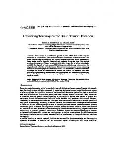
(a)
(b)
Figure 1. Alternative superimposed (a) matrix and (b) node-link visualizations supporting weighted graph comparisons.
ral groupings or anatomically segregated brain regions [26]. Although, the processes for acquiring the two types of connectivity data differ, they can both be expressed as weighted graphs in which nodes represent ROIs and edges can encode the strength of their correlation (functional) or the density of fibers connecting them (anatomical). Recent research in neuroscience successfully began to analyze the connectivity data using graph theoretical methods [20] and statistics [43]. However, visualization systems can provide significant insights for the discovery of unforeseen structural correlation patterns, in particular across several datasets. For example, comparing patterns of functional connectivity and anatomical connectivity pre- and post-removal of parts of brain tissue may help neuroscientists to understand how the brain rewires itself to restore its function. Although statistical and graph theoretical methods are available for such analysis, visualization systems featuring connectivity comparison tools can provide significant insights for the discovery of unanticipated correlation patterns. Visual graph comparison, thus, can be an essential tool for comprehensive brain connectivity analysis. To build effective interfaces for brain connectivity analysis, we identify common visual analysis tasks that neuroscientists carry out in brain connectivity analysis based on interviews with neuroscientists and an in-depth review of the domain literature. By doing so, we provide a link from domain-specific problems in neuroscience to more generic problems in HCI and visualization. Based on this task identification, we also establish that weighted graph comparisons can benefit a group of higher-level tasks in visual brain connectivity analysis. We explored alternative visual encodings that facilitate the comparison of edge weights across two graphs in a superimposed view, both in node-link diagrams and adjacency matrices.
Finally, we report on a controlled experiment comparing two of these representations (Fig. 1) for their ability to encode connection weights of two graphs. Results of the study led us to implications for the design of brain connectivity visualization tools. While weighted graphs are present in a plethora of domains: computer networks, social networks, biological pathways networks, air traffic networks, commercial trade networks; very few tools currently exist to represent and compare them. As we used generic comparison tasks during the study, our results can also inform the design of general weighted graph comparison tools. HIGH-LEVEL BRAIN CONNECTIVITY ANALYSIS TASKS
Neuroscientists investigate brain connectivity to answer questions such as how brain connectivity changes throughout development, with aging, or with physical injury, what kind of connectivity patterns are required for a particular functionality, and how these connectivity patterns show variances across individuals and across certain anomaly conditions. Some of the subtasks carried out during these explorations can be supported by visualizations. Through a literature survey and a series of one-hour long interviews with seven neuroscientists, we identified a list of major tasks in brain connectivity analysis where visualizations are already in use or can be used to aid and enhance the analysis: 1. Identify network structures that are responsible for a specific cognitive function: Neuroscientists examine how our brain carries out specific cognitive functions, identify the regions responsible or involved, and study their interaction with each other while executing these functions [41]. However, significant individual variations exist. These variations require the comparison of connectivity data of large subject groups to be able to identify common network structures. 2. Identify effects of anatomical structure on functional connectivity: Understanding the effect of anatomical structure on the formation of functional relations is a key challenge in neuroscience [9, 24, 25]. For this purpose, scientists look for correlated patterns across anatomical and functional connectivity, requiring the simultaneous exploration of the two connectivity data to reveal complex mappings between. 3. Identify alterations in brain connectivity: Brain connectivity of an individual changes over time—through development and with aging [14]. Another instance of alteration in brain connectivity is the development of re-routings that restore functionality typically after a local injury [10]. In addition, changes in white matter fiber connectivity following behavioral training of a complex skill have also been reported [35]. In order to understand the temporal evolution of these changes, scientists need to compare connectivity data gathered at different instances in time. 4. Identify the existence or the loss of patterns in brain connectivity that are associated with anomalous conditions: Neuroscientists have already shown that certain cognitive anomalies are associated with the loss of specific connectivity patterns [6, 34]. For instance in Alzheimer’s disease, it is observed that functional connectivity does not exhibit small-world properties as much as a healthy brain [34].
Identifying such differences in connectivity patterns is essential for the diagnosis and treatment of these anomalies, which can be done by comparing the connectivity of the anomalous brains to healthy ones. 5. Identify deviation of an individual’s connectivity from a population mean: The aforementioned tasks often utilize an ‘average’ brain—the term ‘average’ encompassing connectivities that are common to all individuals. The average brain, in turn, can be used to characterize an individual’s brain by studying the deviation of it from the average brain. 6. Effective brain parcellation and multimodal connectivity analysis: Identifying brain structures that act as a unit is an important problem. Automatic parcellation algorithms, based on statistical likelihood of synchronized activation, are employed to identify these units. A variety of statistical techniques along with multiple data sources exist each yielding different parcellations. For example, an automatic parcellation based only on functional connectivity data can be refined by taking into account fiber connectivity [29], or anatomy-based parcellation can be validated by functional connectivity relationships between the regions [7]. Thus, different parcellation outcomes are needed to be compared to verify the robustness of a technique [42]. 7. Identify effects of local injury: In clinical applications it is important to predict the effect of a local injury. A localized damage of anatomical structure can have multiple implications on functional connectivity due to the loss of indirect as well as direct connections. Similarly, in image-guided neurosurgery [4], identifying optimal surgical paths that minimize damage induced by intervention is also important. In order to be able to make these decisions, neurologists look at brain connectivity data in a spatial context and observe which anatomical and functional connections are associated with which specific brain locations. This summary shows that a large number of neuroscientific problems can be facilitated with weighted graph comparison tools. Apart from the last task, for which connectivity data has to be presented in its spatial context (inside the brain volume), all other tasks can be conducted with non-spatial representations such as 2D node-link diagrams and adjacency matrices. Although it is essential for brain connectivity analysis to communicate spatial context of the data to ease the interpretation, non-spatial representations can prove more effective for communicating changes in complex connectivity data, as they relax a set of strong constraints on the visual representations (such as preserving the exact shape of connections in three dimensions). Hence, tools supporting brain connectivity analysis have to offer multiple visual representations—each of which are optimal for specific set of tasks. In this paper our focus is on connectivity comparison tasks which, at an abstract level, can be expressed as comparison of two weighted graphs. RELATED WORK
Work relating to our own can be found in three domains: the study of brain connectivity in neuroscience, the use of visualizations within this domain, and research on graph comparison and weighted graph visualizations in information visualization. We review each of these areas below.
Brain Connectivity
Functional connectivity data is derived from functional magnetic resonance imaging (fMRI). Based on the blood oxygen consumption level, fMRI images show active regions of the brain at a given instance. Neuroscientists apply a variety of statistical and computational methods over collections of fMRI images to characterize global structures in the coordinated neural activity [32, 37]. Functional connectivity, therefore, can be seen as a relatedness among specific region of interests (ROIs) in the brain which are highly correlated functionally. Thus, functional connectivity among ROIs can be represented as a fully connected, weighted relatedness graph. White matter fibertracts, the so called anatomical connectivity structures, are derived through applying tractography algorithms to diffusion tensor imaging (DTI) data which represents anisotropic diffusion of water through bundles of neural axons. The resulting fibertracts (representing axon bundles) are often clustered based on their trajectory similarities and regions that they connect to [27]. It is possible to define a fiber connectivity measure between all ROI pairs depending on the fibertract density between them [22]. Hence, similar to functional connectivity, anatomical connectivity between regions of the brain can be expressed as a weighted graph.
(a)
(d)
(b)
(e)
(c)
(f)
Use of Visualizations in Brain Connectivity Analysis
Defined as a correlation matrix between specific locations within the brain volume (ROIs), functional connectivity data is often visualized as 3D node-link diagrams: ROIs are shown as nodes and weighted edges denote the pairwise strength of these node relationships (e. g., Fig. 2(a)). Although the edges below a certain strength threshold can be hidden, the resulting images are still cluttered and suffer from the known side effects of 3D rendering such as occlusion [14, 19]. To facilitate comparison, two connectivity datasets can be overlaid within the 3D brain [42], with edge colors denoting correlation and anti-correlation between the end points. However, the clutter and complexity of the visual encoding in these spatial/volumetric representations makes it difficult to perform accurate weighted edge comparison tasks. An alternative approach is to show the connectivity data as a 2D node-link diagram whose layout is calculated by multidimensional scaling or force-directed algorithms [1] (e. g., Fig. 2(c)). These layouts remedy some of the clutter problems by eliminating overlaps and reducing number of long edges. They are thus adopted especially among those scientists who practice graph-theoretical analysis of brain connectivity. The spatial context of the data, however, is still crucial for an effective interpretation of the data by neuroscientists who are trained to reason with respect to spatial brain regions. Hence, node-link diagrams are often accompanied with a separate spatial rendering of the node positions, with nodes on the two representations being matched by region color and label [31]. To preserve the spatial character of the data to some extent, many 2D connectivity node-link diagrams adopt a biological layout where node positions are projections on 2D planes defined by two of the standard anatomical axes (e. g., ventrodorsal, anteroposterior, left-right; e. g., Fig. 2(b)) [1]. These layouts communicate spatial properties of the data coarsely, helping scientists orient themselves in the graph, while en-
Figure 2. Existing visualization techniques for brain connectivity. Left column, functional connectivity: (a) 3D spatial node-link diagram within the brain volume (courtesy of Erik Ziegler, Cyclotron Research Centre, Univ. of Li`ege, generated with ConnectomeViewer [19]), (b) 2D nodelink diagram with biological layout [1], and (c) force-directed node-link accompanied with a spatial visualization showing actual positions of the nodes [31]. Right column, anatomical connectivity: (d) fibers within the 3D volume of the brain, (e) fiber density ROI graph as a spatial node-link diagram [22], and (f) matrix representation of fiber densities between ROIs [22]. All images reproduced with authors’ permissions.
abling the use of color for encoding other information such as change across two states [6, 33]. Matrices of functional connectivity as an alternative representation are also popular [1, 19, 34] and are occasionally used in the form of small multiples to illustrate trends across different connectivity datasets [5, 20, 28]. To support direct comparisons, correlation coefficients from multiple scan states can be shown within nested quadrants of a matrix cell [39]. However, this design makes it hard to focus on a single scan state. Representing physical entities, fibertracts that constitute anatomical connectivity are more frequently visualized within the 3D brain volume [19] (e. g., Fig. 2(d)). Research in fiber connectivity visualization focuses on their similarity clustering, bundling, and selection in 3D space [30, 38] as well as on illustrative depiction [18]. While non-spatial representations for fiber similarity and clustering are also used [27], neuroscientists reported difficulties with interpreting these representations. Related to our work, anatomical connectivity can be reduced to a fiber density graph among ROIs and vi-
sualized as a 3D spatial node-link diagram combined with a matrix representation [22] (e. g., Fig. 2(e)–(f)). So far, the coordinated visualizations of structural and functional connectivity has received little attention, and existing visualizations focus on spatial representations rather than supporting abstract graph comparison tasks. Several tools (e. g., ConnectomeViewer [19, 29]) support visual brain connectivity analysis using spatial 3D node-link and matrix representations for functional connectivity and volumetric fibertract representations for anatomical connectivity. Although it is crucial to communicate the spatial context in brain connectivity analysis for several tasks, 2D non-spatial representations with flexible layouts are more suitable to communicate differences/changes in the connectivity data in an explicit way. To the best of our knowledge, none of the existing brain connectivity tools supports such a visual connectivity comparison. Weighted Graph Visualization and Comparison
A weighted graph is visualized either as a node-link diagram or an adjacency matrix. In node-link diagrams, weight is either mapped to the length of an edge with inverse proportions [11] or is encoded in the thickness and/or color of an edge [16]. In matrix visualizations, the weight of a connection is mapped either to the color of the corresponding cell or to the size of a glyph inside the cell [40]. Among these representations, people most commonly encode weight as edge thickness in node-link diagrams. However, to the best of our knowledge, there is no study on alternative visual encodings of edge weight for graphs nor their comparison.
VISUALIZATION DESIGN RATIONALE
In the following we discuss our choices for visually coupled presentation of two graphs and visual encodings adopted in node-link and matrix visualizations. Visually Coupled Graph Representations
Comparing two weighted graphs requires communicating absence or presence of connections, as well as their absolute weights in both graphs. As mentioned above, three alternative representations exist for presenting two graphs: side-by-side (juxtaposed), overlaid (superimposed), and animated views. While smooth animations are effective for observing trends over multiple states, they do not provide information about two graphs in a single image. Additionally, smooth animations may increase the time requirement as the viewer may need to watch the animation repeatedly when multiple elements from both graphs need to be compared. Therefore, we only considered side-by-side and overlaid representations. From informal feedback on our initial implementations, sideby-side views proved to be much slower and error-prone compared to the overlaid views—likely due to the fact that the distance to be covered even for simple comparison tasks is much higher in the side-by-side view compared to the overlaid views (element lookup). The difference increases tremendously as the graphs get larger. Moreover, side-by-side views necessitate about double the screen space compared to the overlaid or animated views.
Comparison of weighted graphs is an open research question. However, various comparison techniques are proposed for unweighted graphs in a number of domains for problems related to characterization of metabolic pathways [8, 36], business process models [2] and software evolution [11].
The last alternative, overlaid views has the potential drawback of visual clutter due to added visual elements. However, for the data sizes and densities we consider in this work, we found overlaid representations to be better suited for the effective execution of the comparison tasks. We thus decided to base our visualizations on overlaid views.
We can categorize techniques for comparing unweighted graphs as follows: (i) juxtaposed views where two graphs are presented side-by-side and often complemented with interactive techniques that highlight the matches between the two [2], (ii) superimposed or overlaid views where a single layout is used for both graphs while differing edges and nodes are color coded [2, 17, 23], and (iii) animated views where positions of nodes are interpolated between the two graphs, while added or removed elements are faded in or out respectively [12, 17]. A more detailed categorization of these techniques was presented by Gleicher et al. [21], who also emphasize the continuing necessity of comparison tools in visualization.
The design space for the visualization of weighted graphs is, in fact, limited to the use of color (intensity or hue) or size on edges in node-link diagrams or glyphs inside the cells in matrix visualizations. However, these mappings do not suffice when edge weights from two graphs need to be shown in an overlaid view. Although it is most common to use edge thickness in node-link diagrams for encoding weight, this approach increases the space requirements especially when edges from two graphs need to be shown. Moreover, when node-link diagrams represent dense graphs, it is important to keep edge thickness at a minimum.
Similar techniques exist for depicting dynamic graphs to communicate changes during a graph’s evolution. Work in this area focuses on the preservation of a viewer’s mental map by restricting layout changes across time steps. This approach facilitates the detection of temporal patterns in both animated and multiple juxtaposed views [3, 13]. Although important, these methods do not easily extend to brain connectivity data where mental map preservation involves spatial aspects of the data, hence requires a deterministic biological layout. Nevertheless, weighted graph comparison—a crucial component in brain connectivity analysis—has yet to be addressed.
Edge Weight Visual Encoding in Node-Link Diagrams
We examined two other options for overlaid edge weight encoding. First, we considered two constant width parallel edges with two different color scales—each encoding the edge weight from one graph (Fig. 3(b)). As the alternative, we considered stacking a dashed edge on a normal edge, enabling viewers to see the line underneath the dashed line (Fig. 3(a)). We tried both alternatives with our datasets and found continuous parallel lines to be more legible, especially for dense graphs. Dashed lines caused much change of color through the entire visualization, making the overview seem cluttered and edges of one graph difficult to isolate.
(a)
(b)
(c)
(d)
(e)
(f)
Figure 3. Examples of all visual encodings examined to facilitate the comparison of weighted graphs. Connections more dominant in Graph1:
Connections more dominant in Graph1
Connections more dominant in Graph2:
Connections more dominant in Graph2
Connections with equal strengths:
Connections with equal strengths
Figure 4. Details of the selected edge weight encoding in matrices (left) and node-link diagrams (right) using superimposition.
Edge Weight Visual Encoding in Matrices
Matrix representations which eliminate occlusion problems that degrade node-link diagrams facilitate the encoding of additional information in cells more effectively [15]. Our initial approach for encoding the weight within a matrix cell was to use scaled glyphs such as concentric circles (Fig. 3(c)). Here the radius of the inner circle is mapped to the union weight and change from one graph to the other is mapped to the outer circle radius, while decrease and increase is differentiated by color. We did not pursue this approach further because of the difficulty of identifying a single connectivity state. Besides, when the difference is minimal, the borders produced between inner and outer circles became illegible within the limited cell space. Next, we examined color-coded bar charts shown within the cell to show the absolute weight from each graph (Fig. 3(d)). We eliminated this approach due to the horizontal line patterns it produced and also complicated focusing on weights from one graph at a time. We investigated alternative ways of dividing matrix cells into two regions and using a separate color scheme for each region to encode weight from the corresponding graph. We tried vertical, horizontal, and diagonal divisions (Fig. 3(e)) but they all produced patterns interfering with the cell boundaries of the matrix. Finally, we adopted an inner and outer squares division (Fig. 3(a)) where the edge weight from each graph is mapped to the color density of the corresponding region. We considered this approach useful since it did not obscure the matrix’ grid structure. It also allowed us to use brightness alone to encode weight since it was possible to differentiate graphs based on the spatial encoding (inner vs. outer)—freeing up hue to encode other data attributes. As a natural outcome of this encoding, the amount of change is mapped to the contrast between inner and outer regions of a cell, easily enabling viewers to differentiate regions with high and low change. CONTROLLED STUDY
In this study we investigate the effectiveness (accuracy, task completion time) of the described node-link diagrams and ma-
trices (Fig. 4) when comparing two graphs (G1 , G2 ) with different edge weights. Our goal is to assess how both techniques scale with changing graph sizes and edge densities across different comparison tasks, to inform designs that would utilize both representations. Representative tasks for the study were derived from common tasks in analyzing differences in brain connectivity, as previously described. Techniques
We used the visual encodings described in the previous section for overlaying two graphs in node-link and matrix visualizations. In all techniques, the entire information is shown in one full-screen window without a need to zoom or pan. This design eliminates any confounds due to navigation issues rather than reading of the visual representation to complete the task. 1. Matrix—Overlaid (M): A single adjacency matrix representation shows edge weights in both graphs. Each matrix cell (12 × 12 pixels) contains an inner region encoding the weight of the edge in G1 and an outer region encoding the weight of the edge in G2 (Fig. 5(a)). The absolute weight is mapped to the color brightness for which we used a perceptually linear scaling. A cell with a light inner and dark outer regions indicates an edge with a high weight in G1 and a low weight in G2 . Vice versa, a cell with a dark inner and a light outer region indicates an edge with a high weight in G2 and a low weight in G1 . Since one of our tasks required identifying a specific region, we reordered rows and columns of the matrix to ensure that nodes were placed in the same regions in both the matrix view and the node-link diagram. To provide users with stable representations across all tasks, we used this ordering for all trials. The tradeoff of this ordering is, however, that it did not ensure a close placement of items that need to be compared during other tasks, as other reordering algorithms could have. 2. Node-Link Diagram—Overlaid (NL): A single node-link diagram shows edge weights in both graphs using two parallel edges. Connections that are present in G1 are encoded in green colored edges, while connections that are present in G2 are encoded with the red colored edges (Fig. 5(b)). Thus, a single green edge represents an edge that was only present in G1 , while a single red edge represents an edge that was only present in G2 . The absolute edge weight is encoded using brightness as in the matrix condition, and we ensured that values for the same edge weight had the same brightness. To ensure the generalizability of our results, we eliminated the fixed biological layout alternative and only used a force-directed layout. We made this choice because fixed layouts produce less optimal arrangements with re-
Participants completed this task by browsing each region successively, estimating the region with highest edge weight variation. To avoid confounds in the study, we ensured that all trials presented a region with discernably higher variation than the rest. Participants clicked on a region of their choice. Data
(a)
(b)
Figure 5. Example from our controlled study: node-link and matrix representation of the same data (small, dense) for the region identification.
spect to edge crossings and visual clutter, thus are likely to decrease the performance of node-link diagrams. Tasks
Based on our task analysis in this paper’s second section, we identified three generic comparison tasks that are required for successfully executing high-level brain connectivity comparisons. These tasks require users to assess changes in edge weights at different level of details: from a single element to the overview of a large portion of the data. Below we describe each task and the optimal strategy for achieving it. Assess weight change of a node’s connections (Trend): Given one highlighted node, does the overall edge weight to all of its neighbors decrease or increase from G1 to G2 ? Participants completed this task in three steps: (1) they needed to identify all connections to the highlighted node, (2) they needed to assess the change in weight for each connection, and (3) they needed to estimate the aggregated change for all these connections. To avoid confounds in the study, we made sure all trials exhibited a clear increase or decrease trend. To prevent participants from selecting one option at random, we offered an additional “I don’t know” option and instructed them to select it if their confidence was low. We excluded these trials from the analysis. Assess connectivity of common neighbors (Connectivity): Given two highlighted nodes, how many of their common neighbors in G1 are still common neighbors in G2 ? Participants completed this task in two steps: (1) they needed to find common neighbors, meaning the nodes that are connected to both of the highlighted nodes and (2), among them, they needed to count how many are present in both graphs. Participants selected an option from 0 to 6. Identify the region with most changes (Region): Identify the region showing the most variation between G2 and G1 ? For this task we provided users with simple interaction tools to view regions. In the node-link case, we divided the diagram into a 4 × 4 grid and assigned each node to the region it fell into. As participants moved their mouse pointer on the diagram, the corresponding region boundary appeared in light blue and nodes of the region became highlighted (Fig. 5(a)). In the matrix condition, we used the same 16 regions, ordering the nodes linearly according to the regions they belonged to. As participants moved their mouse pointer on the matrix, the region boundaries were highlighted (Fig. 5(b)).
We used synthetic data in order to ensure generalizability of the results, and to be able to control data size and density. We generated four types of uniform networks with either 40 (Small) or 80 (Large) number of nodes, and with either 5% (Sparse) or 10% (Dense) edge density. For each data type, we created four isomorphic networks per trial which were used across all tasks. We created five additional datasets for training with a Small, Sparse metric. The edge weights were assigned arbitrarily to each of the generated graphs, ranging from 0 to 1 in increments of 0.2. We created comparison graphs by copying the original weighted graphs and then randomly perturbing the edge weights of 70% of the edges in order to ensure edge weights that remain constant across the graphs. Participants and Setting
11 participants (1 female) participated in the study with a mean age of 30.2 years. All participants had normal or correctedto-normal vision, without color deficiency. Participants were graduate students or researchers, familiar with graphs. The experiment was conducted in a quiet room during the day. The study computer was a 2.4 GHz Dual-Core HP Z800 workstation equipped with a 30 inch screen with a 2500 × 1600 pixel resolution. The visualization area was restricted to window of 1500 × 1350 pixels. Participants interacted with a mouse and keyboard to complete the tasks. Experimental Procedure
We used a within-subject, full-factorial design: 2 Techniques × 3 Tasks × 2 Sizes × 2 Densities. We repeated each condition four times. We counter-balanced the techniques (M, NL) using a Latin square. Tasks appeared always in a fixed order of increasing complexity (Trend, Connectivity, and Region). Datasets also appeared in a fixed order from simple (Small and Sparse) to more complex (Large and Dense). For each trial, we measured accuracy and task completion time. Before the controlled experiment, we instructed participants about the visualizations as well as the weight encoding used in each, making sure none of them had any vision problems. We asked them to complete trials as accurate and as fast as possible. Before each new technique and task, five training trials were provided. Participants completed the first two following the explanations of the instructor. They answered the remaining trials on their own unless they had further questions. Trials were not timed during the training. After training trials, participants completed the 16 timed trials (2 Size × 2 Density × 4 Repeat) required for each condition (technique × task). For all conditions, we collected a total of 96 trials per participant (excluding training). To keep the experiment within a reasonable time, we limited the time per trial to 30 seconds (measured as a feasible value in a pilot study) and notified participants before the experiment. After 20 seconds, the screen flashed and a time counter
Hypotheses
Our hypotheses for the experiment were the following: • H1—For the Trend task, we expected Matrix to outperform (accuracy and completion time) Node-Link for high-density datasets. We expected that occlusion problems in NodeLink would get severe in Dense cases, causing more errors. We also believed that the spatial encoding used in Matrix would prove easier to remember than the color encoding used in Node-Link, leading to faster answers. • H2—For the Connectivity task, we expected Matrix not to outperform Node-Link because we believed participants might need to compare two distant columns or rows in Matrix, whereas the force-directed layout in Node-Link ensures that connected nodes are in closer proximity. • H3—For the Region task, we expected Matrix to outperform Node-Link (accuracy and completion time). In Matrix, all connections of nodes in one region are contained within the region boundary. However, in Node-Link, participants had to consider links that are drawn across region boundaries, leading to more errors and slower answers. • H4—Overall, we expected Node-Link to decrease in performance (accuracy and completion time) for Dense datasets, as edge density causes many edge crossings, decreasing the legibility of this representation. Results
We used a repeated-measure analysis of variance (RMANOVA) to analyze the collected accuracy and time performance data. We performed the RM-ANOVA on the logarithm of the task times to normalize the skewed distribution, as is standard practice with reaction time data. The analysis of the time performance is reported for correct answers only. Accuracy. The accuracy results are summarized in Table 1 and Fig. 6(a). We found a significant effect of accuracy for Technique (F(1,10) = 55.32, p < .0001) with a large effect size (η p2 = .85). Overall, Matrix is about 20% more accurate than Node-Link. The RM-ANOVA also revealed a significant effect of Task (F(2,20) = 28.67, p < .0001) with large effect size (η p2 = .74), and a significant effect of the interaction Task Table 1. Means of accuracy in percentages, the standard error is indicated in parentheses. Significant differences in accuracy are indicated by *. More accurate results are highlighted in bold.
All tasks* Trend * Connectivity * Region *
Matrix 88.5 (0.9) 95.5 (1.2) 90.3 (1.0) 79.6 (2.1)
Node-Link 69.3 (2.0) 85.2 (4.3) 70.5 (2.5) 52.3 (4.5)
p-value < .001 < .05 < .0001 < .0001
100
15
80
Mean Accuracy
10
Mean Time
appeared below the visualization for the remaining 10 seconds. To provide their answer, participants pressed the space bar to view the dialog box with the answers. After this point, the timer stopped and the visualization disappeared. Participants were instructed to take breaks if needed when no visualization was shown on the display. None of the participants took a noticable break nor reported any fatigue.
60
40
5
20
0
Trend
Connectivity TASKS
0
Region
(a)
Trend
(b)
Connectivity TASKS
Matrix
Region Node-Link
Figure 6. (a) Mean accuracy in %, (b) and mean completion time in seconds per task for matrix (blue) and node-link (red) techniques. Error bars represent +/– 2 standard errors.
× Technique (F(2,20) = 4.34, p < .05) with a large effect size (η p = .30). Pairwise comparisons revealed that Matrix is more accurate than Node-Link for all three tasks. We also found a significant effect of Size (F(1,10) = 18.69, p < .01) with a large effect size (η p2 = .65) and Density (F(1,10) = 61.00, p < .0001) with a large effect size (η p2 = .86). As expected, accuracy decreases for Large or Dense networks. The interaction Technique × Size (F(1,10) = 6.5, p < .05) is significant with a large effect size (η p2 = .39). Node-Link is affected by Size, losing about 25% accuracy in large datasets compared to small ones. In contrast, Matrix has less than 1% loss in accuracy. Pairwise comparisons indicate that Matrix significantly outperforms Node-Link for large networks across all three tasks. The results indicate that both Techniques are affected by Density, Matrix losing about 10% accuracy, Node-Link about 20%. Pairwise comparisons indicate that Matrix significantly outperforms Node-Link both for Sparse and Dense networks across all three tasks. Completion Time. We analyzed the completion time for correct answers only, using a mixed linear model capable of handling missing data cases. We excluded about 10% incorrect trials for Matrix and 30% for Node-Link (out of 528 total trials per technique). The completion time results are summarized in Table 2 and Fig. 6(b). We found a significant effect of time for Technique (F(1,10) = 28.40, p < .0001). Overall, Matrix is 15% faster than Node-Link. We also found a significant effect of Task (F(2,20) = 183.25, p < .0001) and Technique × Task (F(2,20) = 3.82, p < .05). Pairwise comparisons reveal that Matrix is faster than Node-Link for Connectivity and Region tasks. We also found a significant effect of Size (F(1,10) = 139.19, p < .0001) and Density (F(1,10) = 30.94, p < .0001). As expected, Table 2. Means of completion times (excluding errors) in seconds, the standard error is indicated in parentheses. Significant differences in completion time are indicated by *. Faster results are highlighted in bold.
All tasks* Trend Connectivity * Region *
Matrix 9.3 (0.3) 7.1 (0.3) 11.7 (0.5) 9.1 (0.5)
Node-Link 11.0 (0.4) 8.2 (0.5) 14.3 (0.7) 11.1 (0.7)
p-value < .001 not significant < .0001 < .01
Table 3. User preference (means of ratings from -2-strongly node-link, -1-somewhat node-link, 0-indifferent, 1-somewhat matrix, 2-strongly matrix), the standard error is indicated in parentheses. Significant differences in user preference are indicated by *.
Overall* Trend Connectivity * Region *
Preference 1.25 (0.26) 0.63 (0.38) 1.31 (0.23) 1.36 (0.21)
p-value < .0001 not significant < .0001 < .0001
completion time increases for Large or Dense networks. The interaction Technique × Size (F(1,10) = 9.84, p < .01) is significant. Node-Link is particularly affected by Size. For Large datasets, the completion time increases by about 60% for NodeLink and 40% for Matrix. For Dense datasets, the completion time increases by about 25% for both techniques. User Preference. Users rated their preference on a 5-point scale from -2 (strong preference for Node-Link) to +2 (strong preference for Matrix). We analyzed these ratings using a z-test. Results reported in Table 3 reveals that there is a significant difference in user preference between Techniques. Users preferred Matrix overall (p < .0001). In fact, 7 out of 11 participants ranked Matrix as the most effective representation (maximum rating of 2). Z-test also showed that the user preference was significantly different for the Connectivity (p < .0001) and the Region tasks (p < .0001). For these tasks, Matrix was preferred to Node-Link. DISCUSSION
The results of our controlled experiment indicate that matrix representations are more effective than node-link diagrams for encoding edge weights and performing comparison tasks. While we expected that it would be the case for the Trend (H1) and Region (H3) tasks in the Dense datasets, we were surprised to find significant differences in accuracy across all tasks for both sparse and dense networks. We also did not expect a significant performance difference across techniques for Connectivity (H2). While we did not find any significant difference in completion time for correct answers, the results indicated that matrix outperformed nodelink in accuracy, contradicting (H2). Although we originally thought that comparison in matrices may be error-prone since the rows or columns to be compared may be far away, we in fact observed that the linear arrangement of the matrix allowed people to inspect each of the candidate neighbors successively. In contrast, despite common neighbors being placed closer together in space in the node-link diagram, performance suffered from the less systematic manner to count them, leading to a decrease in accuracy. We did not expect the strong performance decrease of nodelink diagrams for large networks, in addition to dense ones (H4). We believe that this happened because, although we used a fixed edge density, the total number of edges increases quadratically with a linear increase in number of nodes. The total number of links shown in large sparse datasets, thus, is much higher than small sparse datasets. To offer a similar visual complexity in small and large graphs, we could envision to control the edge density per display area unit.
Implications for design
The findings of the study indicate that, for edge weight comparisons, node-link representations are more error-prone and less readable than matrices. However, node-link diagrams offer a flexible layout that can be adjusted to reflect spatial characteristics of the data much more effectively than the linear matrix orderings allow. Therefore, while scientists should adopt matrix representations to ensure better accuracy when performing comparison tasks, efforts have to be made to augment these visualizations with spatial context or couple them with appropriate spatial representations. A second point to consider relates to the datasets’ density. While we tested graphs with connection densities of 5% and 10%, brain connectivity data is, in fact, a fully connected graph with a wide range of weight values; it becomes spare after thresholding: removing edges with weight under a specified threshold. One classical criteria for thresholding is to limit the density of the graph to be readable using a node-link representation. For certain tasks, it may be preferable to analyze the entire connectivity information to spot patterns in weak connections. In such cases, matrix representations are the best choices as they scale better with density. For other cases such as the presentation of key findings, however, node-link diagrams may be a better choice because they are more compact for presenting significant trends and are better at preserving the spatial context. CONCLUSION AND FUTURE WORK
The comparison of brain connectivity patterns is a general problem in the neurosciences. To address it, we have gathered a list of seven tasks that are very common in this domain, both from interviews with experts and from a literature survey, and shown that most of these tasks can be translated to weighted graph comparisons. To support these tasks, we have explored the design space of applicable visual representations. We chose the two most suitable: one augmenting node-link diagrams and the other augmenting adjacency matrices. We thus designed novel visual representations to depict the edges along with the two weights to be compared between graphs. Based on this visualization design we performed a controlled study, comparing the two representations using two graph sizes and two graph densities. The results show that matrices outperform node-links for the chosen tasks, especially when the graph becomes dense or large. Our recommendation is thus that matrices should be used unless the graph is small and sparse. To the best of our knowledge, this paper is the first to present visualizations designed for weighted graph comparison tasks as well as a controlled study of their effectiveness. The tasks that we selected in our study consider the graphs to be non-spatial. Spatial representations, however, are still essential for neuroscientists especially for tasks that rely on spatial locations such as comparing patterns around an injury in the brain. As for future work, we will investigate integration of our proposed non-spatial visualization with spatial visualizations. Since weighted graphs exist in a wide variety of domains such as social and computer networks, we will also investigate other
application areas for our proposed visualization. While some useful tasks for these domains are likely to differ from the ones we considered, we believe our visual representations are still suitable and that our results would still hold, although variations in the visual encodings could certainly improve some particular domain-dependent tasks.
10. Cao, C., and Slobounov, S. Alteration of Cortical Functional Connectivity as a Result of Traumatic Brain Injury Revealed by Graph Theory, ICA, and sLORETA Analyses of EEG Signals. IEEE Transactions on Neural Systems and Rehabilitation Engineering 18, 1 (2010), 11–19. doi> 10.1109/TNSRE.2009.2027704
ACKNOWLEDGEMENTS
11. Collberg, C., Kobourov, S., Nagra, J., Pitts, J., and Wampler, K. A System for Graph-Based Visualization of the Evolution of Software. In Proc. SoftVis, ACM (2003), 77–86. doi> 10.1145/774833.774844
We would like to thank Thomas Grabowski, Jr., MD, Dr. Tara Madhyashta, Dr. Kayo Inoue from The Integrated Brain Imaging Center (IBIC) at University of Washington, and to Dr. Arjun Bansal from Harvard Medical School for their valuable input that went into this work. REFERENCES
1. Achard, S., Salvador, R., Whitcher, B., Suckling, J., and Bullmore, E. A Resilient, Low-Frequency, Small-World Human Brain Functional Network with Highly Connected Association Cortical Hubs. J. Neurosci. 26, 1 (2006), 63–72. doi> 10.1523/JNEUROSCI.3874-05.2006 2. Andrews, K., Wohlfahrt, M., and Wurzinger, G. Visual Graph Comparison. In Proc. IV, IEEE Computer Society (Los Alamitos, 2009), 62–67. doi> 10.1109/IV.2009.108 3. Archambault, D., Purchase, H., and Pinaud, B. Animation, Small Multiples, and the Effect of Mental Map Preservation in Dynamic Graphs. IEEE TVCG 17, 4 (2011), 539–552. doi> 10.1109/TVCG.2010.78 4. Archip, N., Clatz, O., Whalen, S., Kacher, D., Fedorov, A., Kot, A., Chrisochoides, N., Jolesz, F., Golby, A., Black, P., et al. Non-Rigid Alignment of Pre-Operative MRI, fMRI, and DT-MRI with Intra-Operative MRI for Enhanced Visualization and Navigation in Image-Guided Neurosurgery. NeuroImage 35, 2 (2007), 609–624. doi> 10.1016/j.neuroimage.2006.11.060 5. Bassett, D., Brown, J., Deshpande, V., Carlson, J., and Grafton, S. Conserved and Variable Architecture of Human White Matter Vonnectivity. NeuroImage 54, 2 (2011), 1262–1279. doi> 10.1016/j.neuroimage.2010.09.006 6. Bassett, D., Bullmore, E., Verchinski, B., Mattay, V., Weinberger, D., and Meyer-Lindenberg, A. Hierarchical Organization of Human Cortical Networks in Health and Schizophrenia. J. Neurosci. 28, 37 (2008), 9239–9248. doi> 10.1523/JNEUROSCI.1929-08.2008 7. Beckmann, M., Johansen-Berg, H., and Rushworth, M. Connectivity-Based Parcellation of Human Cingulate Cortex and Its Relation to Functional Specialization. J. Neurosci. 29, 4 (2009), 1175–1190. doi> 10.1523/JNEUROSCI. 3328-08.2009 8. Brandes, U., Dwyer, T., and Schreiber, F. Visual Understanding of Metabolic Pathways Across Organisms Using Layout in Two and a Half Dimensions. Journal of Integrative Bioinformatics 1, 1 (2004), 2:1–2:16. doi> 10. 2390/biecoll-jib-2004-2 9. Bullmore, E., and Sporns, O. Complex Brain Networks: Graph Theoretical Analysis of Structural and Functional Systems. Nature Reviews Neuroscience 10, 3 (2009), 186–198. doi> 10.1038/nrn2618
12. Diehl, S., and G¨org, C. Graphs, they are Changing: Dynamic Graph Drawing for a Sequence of Graphs. In Proc. Graph Drawing, Springer (2002), 23–31. doi> 10. 1007/3-540-36151-0 3 13. Diehl, S., G¨org, C., and Kerren, A. Preserving the Mental Map using Foresighted Layout. In Proc. VisSym, Eurographics Association (2001), 175–184. 14. Dosenbach, N., Nardos, B., Cohen, A., Fair, D., Power, J., Church, J., Nelson, S., Wig, G., Vogel, A., Lessov-Schlaggar, C., et al. Prediction of Individual Brain Maturity Using fMRI. Science 329, 5997 (2010), 1358–1361. doi> 10.1126/science.1194144 15. Elmqvist, N., Do, T.-N., Goodell, H., Henry, N., and Fekete, J.-D. ZAME: Interactive Large-Scale Graph Visualization. In Proc. PacificVIS, IEEE Computer Society (2008), 215–222. doi> 10.1109/PACIFICVIS.2008. 4475479 16. Epskamp, S., Cramer, A., Waldorp, L., Schmittmann, V., and Borsboom, D. qgraph: Network Visualizations of Relationships in Psychometric Data. Journal of Statistical Software 48, 4 (2012), 1–18. 17. Erten, C., Harding, P., Kobourov, S., Wampler, K., and Yee, G. GraphAEL: Graph Animations with Evolving Layouts. In Proc. Graph Drawing, Springer (2004), 98–110. doi> 10.1007/978-3-540-24595-7 9 18. Everts, M. H., Bekker, H., Roerdink, J. B. T. M., and Isenberg, T. Depth-Dependent Halos: Illustrative Rendering of Dense Line Data. IEEE TVCG 15, 6 (2009), 1299–1306. doi> 10.1109/TVCG.2009.138 19. Gerhard, S., Daducci, A., Lemkaddem, A., Meuli, R., Thiran, J., and Hagmann, P. The Connectome Viewer Toolkit: An Open Source Framework to Manage, Analyze, and Visualize Connectomes. Frontiers in Neuroinformatics 5 (2011), 3:1–3:15. doi> 10.3389/fninf. 2011.00003 20. Ginestet, C., and Simmons, A. Statistical Parametric Network Analysis of Functional Connectivity Dynamics during a Working Memory Task. NeuroImage 55, 2 (2011), 688–704. doi> 10.1016/j.neuroimage.2010.11.030 21. Gleicher, M., Albers, D., Walker, R., Jusufi, I., Hansen, C., and Roberts, J. Visual Comparison for Information Visualization. Information Visualization 10, 4 (2011), 289–309. doi> 10.1177/1473871611416549
22. Hagmann, P., Cammoun, L., Gigandet, X., Meuli, R., Honey, C., Wedeen, V., and Sporns, O. Mapping the Structural Core of Human Cerebral Cortex. PLoS Biology 6, 7 (2008), e159. doi> 10.1371/journal.pbio.0060159 23. Hasco¨et, M., and Dragicevic, P. Interactive Graph Matching and Visual Comparison of Graphs and Clustered Graphs. In Proc. AVI, ACM (2012), 522–529. doi> 10.1145/2254556.2254654 24. Honey, C., K¨otter, R., Breakspear, M., and Sporns, O. Network Structure of Cerebral Cortex Shapes Functional Connectivity on Multiple Time Scales. PNAS 104, 24 (2007), 10240–10245. doi> 10.1073/pnas.0701519104 25. Honey, C., Sporns, O., Cammoun, L., Gigandet, X., Thiran, J., Meuli, R., and Hagmann, P. Predicting Human Resting-State Functional Connectivity from Structural Connectivity. PNAS 106, 6 (2009), 2035–2040. doi> 10. 1073/pnas.0811168106 26. Horwitz, B. The Elusive Concept of Brain Connectivity. Neuroimage 19, 2 (2003), 466–470. doi> 10. 1016/S1053-8119(03)00112-5 27. Jianu, R., Demiralp, C., and Laidlaw, D. Exploring 3D DTI Fiber Tracts with Linked 2D Representations. IEEE TVCG 15, 6 (2009), 1449–1456. doi> 10.1109/TVCG.2009.141 28. Kramer, M., Eden, U., Lepage, K., Kolaczyk, E., Bianchi, M., and Cash, S. Emergence of Persistent Networks in Long-Term Intracranial EEG Recordings. J. Neurosci. 31, 44 (2011), 15757–15767. doi> 10.1523/JNEUROSCI.2287-11. 2011 29. Li, K., Guo, L., Faraco, C., Zhu, D., Chen, H., Yuan, Y., Lv, J., Deng, F., Jiang, X., Zhang, T., et al. Visual Analytics of Brain Networks. NeuroImage 61, 1 (2012), 82–97. doi> 10.1016/j.neuroimage.2012.02.075 30. Moberts, B., Vilanova, A., and van Wijk, J. Evaluation of Fiber Clustering Methods for Diffusion Tensor Imaging. In Proc. Visualization, IEEE Computer Society (2005), 65–72. doi> 10.1109/VISUAL.2005.1532779 31. Nelson, S., Cohen, A., Power, J., Wig, G., Miezin, F., Wheeler, M., Velanova, K., Donaldson, D., Phillips, J., Schlaggar, B., and Petersen, S. A Parcellation Scheme for Human Left Lateral Parietal Cortex. Neuron 67, 1 (2010), 156–170. doi> 10.1016/j.neuron.2010.05.025 32. Rajapakse, J., and Zhou, J. Learning Effective Brain Connectivity with Dynamic Bayesian Networks. NeuroImage 37, 3 (2007), 749–760. doi> 10.1016/j. neuroimage.2007.06.003 33. Richiardi, J., Eryilmaz, H., Schwartz, S., Vuilleumier, P., and Van De Ville, D. Decoding Brain States from fMRI Connectivity Graphs. NeuroImage 56, 2 (2011), 616–626. doi> 10.1016/j.neuroimage.2010.05.081
34. Sanz-Arigita, E., Schoonheim, M., Damoiseaux, J., Rombouts, S., Maris, E., Barkhof, F., Scheltens, P., and Stam, C. Loss of ‘Small-World’ Networks in Alzheimer’s Disease: Graph Analysis of fMRI Resting-State Functional Connectivity. PloS one 5, 11 (2010), e13788. doi> 10.1371/journal.pone.001378 35. Scholz, J., Klein, M., Behrens, T., and Johansen-Berg, H. Training Induces Changes in White-Matter Architecture. Nature Neuroscience 12, 11 (2009), 1370–1371. doi> 10. 1038/nn.2412 36. Schreiber, F. Comparison of Metabolic Pathways using Constraint Graph Drawing. In Proc. APBC, Australian Computer Society, Inc., Australian Computer Society, Inc. (2003), 105–110. 37. Seth, A. A MATLAB Toolbox for Granger Causal Connectivity Analysis. J. Neurosci. Methods 186, 2 (2010), 262–273. doi> 10.1016/j.jneumeth.2009.11.020 38. Sherbondy, A., Akers, D., Mackenzie, R., Dougherty, R., and Wandell, B. Exploring Connectivity of the Brain’s White Matter with Dynamic Queries. IEEE TVCG 11, 4 (2005), 419–430. doi> 10.1109/TVCG.2005.59 39. Thomason, M., Dennis, E., Joshi, A., Joshi, S., Dinov, I., Chang, C., Henry, M., Johnson, R., Thompson, P., Toga, A., Glover, G. H., Horn, J. D. V., and Gotlib, I. H. Resting-State fMRI Can Reliably Map Neural Networks in Children. NeuroImage 55, 1 (2011), 165–175. doi> 10. 1016/j.neuroimage.2010.11.080 40. van Ham, F., Schulz, H., and Dimicco, J. Honeycomb: Visual Analysis of Large Scale Social Networks. In Proc. INTERACT, Springer (2009), 429–442. doi> 10. 1007/978-3-642-03658-3 47 41. Vidal, J., Freyermuth, S., Jerbi, K., Hamam´e, C., Ossandon, T., Bertrand, O., Minotti, L., Kahane, P., Berthoz, A., and Lachaux, J. Long-Distance Amplitude Correlations in the High Gamma Band Reveal Segregation and Integration within the Reading Network. J. Neurosci. 32, 19 (2012), 6421–6434. doi> 10. 1523/JNEUROSCI.4363-11.2012 42. Worsley, K., Chen, J., Lerch, J., and Evans, A. Comparing Functional Connectivity via Thresholding Correlations and Singular Value Decomposition. Philos. Trans. R. Soc. Lond. B Biol. Sci. 360, 1457 (2005), 913–920. doi> 10.1098/rstb.2005.1637 43. Zalesky, A., Fornito, A., and Bullmore, E. Network-Based Statistic: Identifying Differences in Brain Networks. NeuroImage 53, 4 (2010), 1197–1207. doi> 10. 1016/j.neuroimage.2010.06.041