Weighted Median Filters - CiteSeerX

IEEE TRANSACTIONS ON CIRCUITS AND SYSTEMS-11:

ANALOG AND DIGITAL SIGNAL PROCESSING, VOL. 43, NO. 3, MARCH 1996

157

Circuits and Systems Exposition Weighted Median Filters: A Tutorial Lin Yin, Ruikang Yang, Member, IEEE, Moncef Gabbouj, Senior Member, IEEE, and Yrjo Neuvo, Fellow, IEEE

Abstract- Weighted Median (WM) filters have attracted a and optimize the designs. A good underlying theory covering growing number of interest in the past few years. They inherent a subclass of nonlinear filters is needed for the research to have the robustness and edge preserving capability of the classical a common foundation and for the methods to be transferable median filter and resemble linear FIR filters in certain properties. Furthermore, WM filters belong to the broad class of nonlinear among applications. A nonlinear filter class that has been proven very useful is filters called stack filters. This enables the use of the tools developed for the latter class in characterizing and analyzing the class of median based filters. During the last few years their the behavior and properties of WM filters, e.g. noise attenuation theory has also been developing quite fast. It is the opinion capability.The fact that WM filters are threshold functions allows of the authors that median based filters today give one sound the use of neural network training methods to obtain adaptive W M filters. In this tutorial paper we trace the development of approach to nonlinear filtering. The success of median filters the theory of W M filtering from its beginnings in the median is based on two intrinsic properties: edge preservation and filter to the recently developed theory of optimal weighted median efficient noise attenuation with robustness against impulsivefiltering. The following one and multidimensional applications type noise, Neither property can be achieved by traditional are presented in this paper: idempotent weighted median filters linear filtering techniques without resorting to time-consuming for speech processing, adaptive weighted median and optimal weighted median filters for image and image sequence restora- and often ad hoc data manipulations. Edge preservation is tion, weighted medians as robust predictors in DPCM coding essential in image processing due to the nature of visual and Quincunx coding, and weighted median filters in scan rate perception. Edges also occur in biomedical signals when the conversion in normal TV and HDTV systems. “system” moves from one state to another. In addition to being able to effectively eliminate impulsive noise, encountered, e.g., in communications systems and TV images [52], [76], it is worth noting that the median filter is the optimal filter for I. INTRODUCTION INEAR filters have been the dominating filter class biexponential noise in a similar manner as the sliding average through the history of signal processing, due mainly to is for Gaussian noise. The median filter is not, however, a perfect filtering opthe sound theoretical basis provided by the theory of linear eration nor it is very flexible. It may cause edge jitter [11], systems and the computational efficiency of linear filtering streaking [12] and may remove important image details [2], algorithms. Despite the elegant linear system theory, not all [66]. The main reason is that the median filter uses only signal processing problems can be satisfactorily addressed through the use of linear filters. Linear filters tend to blur rank-order information of the input data within the filter sharp edges, fail to remove heavy tailed distribution noise window, and discards its original temporal-order information. effectively, and perform poorly in the presence of signal- For constant signals embedded in i.i.d. noise, temporal-order is dependent noise [78], [79]. Many researchers seem to have irrelevant. This, however, is not true for nonconstant signals the view that it is difficult to obtain major breakthroughs corrupted by noise [72]. In order to utilize both rank- and in signal processing without resorting to nonlinear methods. temporal-order information of input data, several classes of Neural networks serve as an example of the potential of the rank order based filters have been developed in recent years, such as FIR-median hybrid (FMH)filters [40], [66], [45], LZ nonlinear approach. On the other hand, due to the lack of sound underlying filters [53], [72], weighted median (WM) and weighted order theory, nonlinear methods tend to be ad hoc and application statistics (WOS) filters [131, [42], [51], [981, 11041, 11151, specific making it very difficult to assess their performance [120], [123], stack filters [16], [24], [27], [541, [581, [811, [911, [98], [113], [125], and Boolean filters [lo], [411, [ S I , [1191. FMH filters and Ll filters make use of the desirable properties Manuscript received March IO, 1994; revised November 1, 1995. This paper of both linear filters and median filters. Several surveys have was recommended by Associate Editor S. Kiaei. L. Yin and R. Yang are with the Nokia Research Center, Tampere, Finland. been written to trace the development from median to stack M. Gabbouj is with the Department of Information Technology, Pori filtering, see for instance, [18], [19], [301, [321. Tampere University of Technology, Finland. Other advances in this area brought about the development Y. Neuvo is with Nokia Mobile Phones R&D Center, Espoo, Finland. of Vector Median filters and Matched Median filters [5], [6]. Publisher Item Identifier S 1057-7130(96)02269-0.

L

1057-7130/96$05.00 0 1996 IEEE

158

IEEE TRANSACTIONS ON CIRCUITS AND SYSTEMS-I1

The vector median was introduced for multispectral signal processing to utilize correlation between different components [5]. Multispectral satellite images and color images in TV systems are typical examples. Vector median filters have been applied for impulsive noise attenuation in color images and cross luminance and cross color elimination [70], [71]. Matched median filters were introduced for detection in communication systems and defined both for baseband and passband systems [6], [loll. It was shown that the matched median filter outperforms the linear matched filter in the case of binary antipodal signaling under impulsive noise. In this paper, we will concentrate on WM filters which are the simplest rank order based filters among those mentioned above. An N-length WM filter can be described by N parmeters and implemented using a sorting operation with the same order of computations as the same size median filter. On the other hand, WM filters offer much greater flexibility in design specifications than the median filter. The weights control the filtering behavior. The relation of WM filters to the median filter is comparable to that of linear FIR filters to the average filter. The aim of this paper is to summarize the recent developments in the theory and applications of WM filtering. In Section 11, median and WM filters are introduced. Some very useful deterministic and statistical properties of median filters are summarized in the same section, and the analogy between WM filters and linear FIR filters is highlighted. In Section 111, the connection between WM filters and Positive Boolean Functions (PBF) is reviewed under the threshold decomposition framework. Section IV explores the main deterministic and statistical properties of WM filters. The problem of optimal design of WM filters is addressed in Section V. An important extension of WM filters, FIR-WOS hybrid filters are reviewed in Section VI. Several I-, 2-, and 3-D applications of WM filters are outlined in Section VU, ranging from speech processing to image sequence processing. Section V m contains some conclusions. Interested readers are referred to the extensive bibliography for more detailed discussions about the theory, extensions, and applications of WM and related filters.

ANALOG AND DIGITAL SIGNAL PROCESSING, VOL 43, NO. 3, MARCH 1996

+ 1, the filtering procedure is denoted as Y ( n )= MED[X(n K ) ,. . . , X ( n ) ,. . . , X ( n + K ) ] (2.1)

length is N = 2K

-

where X ( n ) and Y ( n )are the nth sample of the input and output sequences, respectively. In most cases, it is reasonable to assume that the signal is of finite length, say L, consisting of samples from X ( 0 ) to X ( L - 1).To be able to filter also the outmost input samples, where parts of the filter window fall outside the input signal, the latter is appended to the required size. The appending of the input signal is commonly performed by replicating the outmost input samples as many times as needed. This appending strategy is referred to as the first and last values carry-on appending strategy, in the literature [29], and will be used throughout the paper. An immediate extension of the median filter is the class of rank order filters. These filters operate exactly like the median filter except that they put out the ith largest sample in the window, the median being a special case Y ( n )=ith largest value of the set [ X ( n- K ) ,. . . , X ( n ) ,. . . , X ( n

+ K ) ] . (2.2)

Two special rank order filters are the minimum and the maximum filters which output the minimum value and the maximum value in the window, respectively. These two operators are the fundamental operations in discrete morphological filtering, with flat structuring elements, namely erosion and dilation [34], [621, [63], [84]. Another simple extension of the median filter is the recursive median filter [69]. The recursive median of window with 2K 1 is defined by replacing some of the input samples in (2.1) by previously derived output samples as follows:

+

+

Y ( n )=MED[Y(n- K ) , Y ( n K l),... , Y ( n- l ) , X ( n ) ,. . . , X ( n + K ) ] .

(2.3)

In recursive median filtering, the filtering operation is performed “in-place” SO that the output of the filter replaces the old input value before the filter window is moved to the next position. With the same amount of operations, the recursive median filter usually provides better smoothing capability than the nonrecursive filter, at the expense of increased distortion. 11. MEDIANAND WEIGHTED MEDIAN FETERS Frequency analysis and impulse response have no meaning Following a brief discussion of the basic deterministic and in median and rank order filtering; the impulse response of a statistical properties of median filters, WM filters are formally median filter is zero! As a result, new tools had to be developed defined and an interesting analogy is drawn between the latter to analyze and characterize the behavior of these nonlinear and linear FIR filters. filters, deterministically and statistically. The basic descriptor of the deterministic properties of median filters is their root A. Median Filtering signal set, that is a set of signals which are invariant to further In an abstract published in EASCON’74, J. Tukey men- filtering. The basic statistical descriptor of median filters is the tioned the “mnning” median as one of those scale invariant set of output distributions which are used to study the noise nonlinear smoothers which might be useful in smoothing time attenuation properties of median filters. These properties of series [92]. Since then, numerous papers, monographs, book median filters are briefly reviewed next. I ) Deterministic Properties of Median Filters: Root Signals: chapters (see for instance [22], [32], [78], [94]) have explored the median operation, analyzing its behavior and proposing Since the output of the median filter is always one of the new and viable extensions. To compute the output of a median input samples, it is conceivable that certain signals could pass filter, an odd number of sample values are sorted, and the through the median filter unaltered. This has been shown to middle or median value is used as the filter output. If the filter hold for median and many medmn-based filters. Since these

159

YIN et al.: WEIGHTED MEDIAN FILTERS

other than the median filter, are constant signals, i.e., trivial. Recursive median filters do also possess the convergence property. Furthermore, they are idempotent, i.e., they produce root signals after a single pass. A recursive median filter has X ( n ) =MED[X(n-K),...,X(n),**.,X(n+K)] . (2.4) exactly the same set of root signals as the (nonrecursive) median filter of the same window width, but a given input If the above condition is satisfied for all n, X ( n ) is called a signal may be filtered to different roots by the two filters. Root root signal of that particular median filter. signals of median related filters have been used for speech and The fact that some signals are invariant to median filtering image coding in [3] and [4], [96], [97]. offers interesting possibilities. In noise filtering, a problem 2) Statistical Properties of Median Filters: Median filters is often how to preserve some desired signal features while are used as robust smoothen and the filtering results are often attenuating noise. An optimal situation would arise if the filter evaluated in a qualitative way. The performance of the filters could be designed so that the desired features were invariant to depends on how well it can suppress undesired parts of the the filtering operation and only noise would be affected. Since signal and, equally important, how well desired information i s the median filter i s a nonlinear filter, and the superposition retained. There is no general numerical measure to combine principle does not apply, this of course can never be fully these two properties and thus evaluate the performance of obtained. However, when a signal consists of constant areas the filter. In the case of linear filters, the two objectives can and stepwise changes between these areas, a similar effect is be achieved if and only if the noise and the signal occupy achieved. Noise will be attenuated, but stepwise changes will different frequency bands. remain. In image filtering, a common approach is to design a The recently developed tools make the analysis of the median filter such that certain image patterns, e.g., lines, are statistical behavior of median filters possible. Assuming that root signals and thus not disturbed by the filtering operation. the samples inside the filter window are a combination of The characterizationof root signals is based on local signal a constant (desired) signal corrupted by some additive white structures, as defined in [33] and [93]. Those used in [33] noise, as done often in the analysis of linear filters, one can are summarized here for a median filter of window width evaluate the output distribution of the filter and hence estimate N = 2K+1. the output variance. Filter optimization is possible based on A constant neighborhood is a region of at least K 1 this approach, but yields even better results when combined consecutive identically valued samples. with other types of constraints (e.g., structural constraints on An edge is a monotonically rising or falling set of samthe filter’s behavior [27]) and applied to extensions of median ples surrounded on both sides by constant neighborhoods of filters which allow much more design flexibility than just the different values. filter length. We shall first review these statistical properties An impulse is a set of at most K samples whose values are of median filters and later those of weighted median filters. different from the surrounding regions and whose surrounding Let the input signal of a median filter be white noise, regions are identically valued constant neighborhoods. modeled here by independent identically distributed random An oscillation is any signal structure which is not part of variables with mean p and variance c2. The corresponding a constant neighborhood, an edge or an impulse. distribution and density functions are denoted by @(t)and Note that the definition of these concepts is tied to the filter #(t),respectively. Results from probability theory [60] give length, e.g., a constant neighborhood of a length N filter is also the distribution, q m e d ( t ) , and the density, $ m p d ( t ) , of the a constant neighborhood for all filters of lengths less than N. median filter output as With these concepts, Gallagher and Wise proved that an arbitrary finite length signal is a median root if it consists of constant neighborhoods and edges only [33] (see also Tyan [93]). They also proved that repeated median filtering of any finite length signal will result in a root signal after and a finite number of passes. This property of median filters is very significant and is called the “convergence property”. The tightest known bound on the number of passes of the median respectively. These two expressions provide the basis for filter necessary to reach a root can be found in [100]: if the quantitative analysis of the noise attenuation of median filters. filter window width i s 2K 1 and the signal has length L, Usually, numerical methods must be used to apply these then at most equations. Under some general assumptions, see [20], the asymptotic distribution (for large N) of the median filter output, when the 3[ 2(K L - 22 )] input is white noise, is normal with mean PL,,d and variance signals define the signature of a filter, they are referred to as root signals. For a median filter of length N = 2K 1 , this means that

+

+

+

+

passes of the filter are required to produce a root signal. This bound is rather conservative in practice. Typically, after 5-10 filterings only slightly, if any, changes take place. All rank order filters possess the convergence property of the median filter. However, all root signals of rank order filters,

2 *medt pmed

= t0.5

(2.7)

,

IEEE TRANSACTIONS ON CIRCUITS AND SYSTEMS-I1

160

ANALOG AND DIGITAL SIGNAL PROCESSING, VOL. 43, NO. 3, MARCH 1996

TABLE I X1 ASYMPTOTIC (FOR LARGE N) OUTPUTVARIANCES OF THE AVERAGE AND THE MEDIANFILTERS OF LENGTH N FOR DIFFERENT INPUT NOISEDISTRIBUTIONS. INPUT IS WHITE NOISEWITH ZERO MEANAND U* VARIANCE Noise probability density

1

Average Median

I

Uniform

I

I

Y

x2

__c_)

Output Signal *N W N

Fig. 1 Gaussian

1

B. Weighted Median Filters

-2

0(.) = --T

me 2o

I

I

Laplacian

4(z)

= -e

1

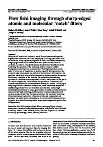
Weighted median filter.

-

v47

where to 5 is defined by Q ( t 0 . 5 ) = 0.5. This result explains the robust noise smoothing properties of the median filter. Regardless of the input distribution, the median operation produces an unbiased estimate of the distribution median t o . 5 . Moreover, the estimate is always consistent, i.e., limN+m eked = 0. The output variance does not depend on the input variance directly, but on 4(to 5) instead. With heavy-tailed or impulsive noise distributions, the variance of the distribution grows with the amplitude of the impulses, whereas q5(to.5) does not necessarily change. Note that the sample mean does not possess this property. Table I lists asymptotic output variances for some common probability distributions. The results for the average filter and the median filter, for uniform noise, are valid for all values of N . Note, that in the case of Laplacian noise distribution, the asymptotic variance of the median operation is half of that of the sample average, i.e., the sample average is 3 dB worse than the median. Also note that for Gaussian noise, the median is only about 2 dB worse than the average. The good performance of the median filter with Laplacian distributed noise is due to an important optimality property of the median operation. The sample median is the maximum likelihood estimate for the location parameter of the Laplacian density. This property shows that the median filter is optimal in the mean absolute error sense for attenuating double exponentially distributed noise. This analogy results from alternate definitions for the average and the median of N values XI, . . . , X N . Consider the expression

The median of X I , . . . , X N can be defined as the value p minimizing L(P) in (2.9) when y = 1. The definition always produces one of the samples X , as a result. The sample average minimizes the same expression when y = 2.

The weighted median (WM) filter was first introduced as a generalization of the standard median filter, where a nonnegative integer weight is assigned to each position in the filter window [13], [51]. In this subsection, we give two alternative definitions of WM filters and discuss the analogy between WM filters and linear FIR filters. As shown in Fig. 1, the structure of a WM filter is quite similar to that of a linear FIR filter. For real-valued signals, WM filters can be defined in two different but equivalent ways. The first definition can be used in the common case of positive integer weights. Dejinition 2.1: For the discrete-time continuous-valued input vector X = [XI,X z , . . . ,X,], the output Y of the WM filter of span N associated with the integer weights

w =[Wl,WZ,...,WNj

(2.10)

is given by

w,0x2,. . . , WNoxjy]

Y = MED[WI 0x1,

-

(2.11)

where MED[.] denotes the median operation and o denotes duplication, i.e., K

times

K o X =X,..., X .

(2.12)

This filtering procedure can be stated as follows: sort the samples inside the filter window, duplicate each sample X , to the number of the corresponding weight W, and choose the median value from the new sequence. Example 2.1: Consider a length 5 WM filter with integer weights [l, 2, 3 , 2, 11. Now apply the filter to the following sequence so that the window is centered at the sample value 8, X 1[-1,5,8,11, -21.

After sorting and duplication, the samples inside the filter window are 11, 11, 8, 8, 8, 5, 5, -1, -2. The filter output is Y = 8, whereas, the 5-point median would have produced the result Y = 5 . The second definition of the WM operation also allows positive noninteger weights to be used. Dejinition 2.2: The weighted median of X is the value p minimizing the following expression N

WlX%- PI.

L(P)= z=1

(2.13)

YIN et al.: WEIGHTED MEDIAN FILTERS

161

TABLE I1 WEIGHTED MEDIANFILTERSFOR WINDOWWIDTH1 THROUGH 5

3

integer weights). The WOS filter has some special properties compared to the WM filter. For example, some WOS filters called asymmetric median filters can eliminate negative impulses (or positive impulses), but preserve positive impulses (or negative impulses) [98]. WM filters can also operate recursively. The output of a recursive WM filter is given by

+

Y (n) =MED[W-K o Y (TI, - K 1), . . . , W-10 Y ( n - 1 ) , W ~ o X ( n ) , . . . , W ~ o X.( n + K ) ] (2.15)

P

is guaranteed to be one of the samples X , because L ( p ) is piecewise linear and convex, if W, 2 0 for all i . The output of the WM filter for real positive weights can be calculated as follows: sort the samples inside the filter window; add up the corresponding weights from the upper end of the sorted set until the sum just exceeds half of the total sum of N weights (i.e., 2 $ W t ) ;the output of the WM filter is thk sample corresponding to the last weight added. Example 2.2: Consider a length 5 WM filter with weights W and an input X: Here,

W=[O.1,0.2,0.3,0.2,0.1],

Recursive WM filters have a certain similarity to linear IIR filters. Although useful in practice, they are in general difficult to handle theoretically. 1)Analogy Between WM Filters and Linear FIR Filters: As the median filter is analogous to the average filter, there exists an interesting analogy between WM filters and linear FIR filters. Let H,, i = 1,2, , N , be the impulse response coefficients of a 1-D FIR filter of size N . If H , 2 0 for all 2, 1 5 i 5 N and E,"=, H , = 1 then the output Y of the FIR filter can be calculated also as

&=[1,5,8,11,2].

After sorting, we get the sorted input set with the corresponding weights

0.2 0.3 0.2 0.1 0.1 1 1 8 5 2 1 Starting from the left, add the weights until the sum reaches or exceeds 0.45. The first weight is smaller than 0.45, so add the next weight. The sum is now 0.5 exceeding 0.45. The weighted median is therefore 8. One fact must be emphasized that there is only a finite number of WM filters for a given finite length window, even though there exists an infinite number of real weight vectors [14], [67]. As already indicated by the above two examples, multiplying the weights by a positive constant does not change the filter. For a detailed treatment of WM filters, particularly with real weights, interested readers are referred to [67]. In particular, it was shown that any real-weight WM corresponds (is identical) to an integer weight WM. Table I1 lists all WM filters for window width 1 through 5 , excluding weight permutations. The number of WM filters grows very rapidly with the window size. For instance, there are 114 WM filters for window width 7, and 172 958 WM filters for window width 9. As the median filter is extended to a rank order filter, the WM filter can be extended to a weighted order statistic (WOS) filter [98]. DeJinifion2.3: For the discrete-time continuous-valued input & = [ X I ,X Z ,. . . , X N ] ,the output Y of the WOS filter of span N associated with the weights and the threshold Th is given by

Y = T h :th largest element of the set [Wl 0 X i , Wz 0 X z , . . . ,WNo X N ] . (2.14) Note that the WM filter is a WOS filter with the same weights and a threshold Th = W, (Th = $ ( l +ELl W 2 )for

N

Y=

H,X, = average(Wlox1,

WZ

0x2,

2=1

(2.16) where W,, 1 5 i 5 N , are positive integers such that H , = W2/ W,. If we replace the average in (2.16) with the median then the definition of the WM filter is obtained. As mentioned earlier, the median is the maximum likelihood estimate of the signal level in the presence of uncorrelated additive biexponentially distributed noise; while, the arithmetic mean is that for Gaussian distributed noise. This means that the sample median of Ar2, i = 1, . . . , N , is the value p which minimizes (2.17) when y = 1 and the sample mean is the value p which minimizes (2.17) when y = 2: N

IX, - PIY.

L(P)=

(2.17)

2=1

If we introduce weights W, in (2.17) as follows: N

WZlXt - PIY

L(P) =

(2.18)

2=l then, in the case y = 2, the value /3 minimizing (2.18) can be expressed as N

P=

N

WtX2I 2=1

w 2

(2.19)

2-1

which can be taken as a normalized FIR filter, i.e., a weighted average. Likewise, if y = 1, the value p minimizing (2.18) is ,8

MED[Wl o X i , *

*

, WNo X,]

i.e., a weighted median. In the sequel, other interesting analogies will be drawn between WM filters and FIR filters. The similarity between them may suggest that WM filters would play as a fundamental role among median type filters as FIR filters among linear filters.

IEEE TRANSACTIONS ON CIRCUITS AND SYSTEMS-I1

162

111. THRESHOLD DECOMPOSITION WEIGHTED MEDIANFILTERS

AND

In 1984, a powerful theoretical tool called threshold decomposition for analyzing rank order based filters was developed by Fitch et al [26]. Using this tool, the analysis of rank order based filters reduces to studying their effects on binary signals.

A. Threshold Decomposition and Median Filtering in the Binary Domain

ANALOG AND DIGITAL SIGNAL PROCESSING, VOL. 43, NO. 3, MARCH 1996

analyze than multivalued signals. The median operation on binary samples reduces to a simple Boolean operation. For example, if the samples inside a length-three binary median filter are denoted by 51, 52, and 53; then the median filter is equivalent to the Boolean expression ZIZZ 2253 21x3 where denotes the logical OR operation and x,xJ is the logical AND operation of variables z, and z J . The approach of threshold decomposition and binary filtering has led to a general class of nonlinear filters called stack filters [98], whose output is given by

+

+

Threshold decomposition of an M-valued signal vector the samples are integer-valued, 0 5 Xi < M , means decomposing it into M - 1 binary signal vectors, g 2 ,. . . ,g"-l, according to the following rule

+

X,where

This thresholding scheme can be applied also to noninteger signals or, in general, to any signal which is quantized to a finite number of arbitrary levels. Example 3.1: Consider a five-valued integer signal vector X = [0,0,2,3,3,3,2,1,0,4,0,1,0,0].

The threshold decomposition of this signal vector into four binary signal vectors results in

(3.5) m=1

where f (.) is a Boolean function which satisfies the stacking property. A Boolean function f possesses the stacking property if whenever two input vectors and 2 stack, i.e., U , 2 v, for each i E { 1,. . . , N } , then also their respective outputs stack, f ( g ) 2 f ( 2 ) . A binary function possesses the stacking property if and only if it can be expressed as a Boolean expression which contains no complements of input variables [35]. Such functions are called positive Boolean functions (PBF's).

z4= [O, 0, 0, 0, 0, 0, 0 , 0 , 0,1,0,0,0,01,

B. Weighted Median Filters and Linearly Separable SeEfdual PBF

xz = [0,0,1,1,1,1,1,0,0,1,0,0,0,0],

WM filters belong to the class of stack filters. In other words, any WM filter can be represented by a PBF in the = [I,2,3,2,1] binary domain. For example, the WM filter corresponds to the following PBF in the binary domain

-

5'

f(Z1,22,53,24,25)

= [0,0)1,1,1,1,1,1,0,1,0,1,0,0].

22x3 f

The original multivalued signal samples X,'s can be reconstructed from the threshold levels by adding these together M-1

xr,

X, =

(3.2)

m=l where X , is the ith sample of X. A very important property of median filters was observed by Fitch et al. [26]: Applying a median filter to an M-valued signal is equivalent to decomposing the signal to M - 1binary threshold signals, filtering each binary signal separately with the corresponding binary median filter, and then adding the binary output signals together. That is, if the multivalued input samples X = [XI,. . . , X,] are inside the median filter window, then the multilevel median output M-1

Y = MED[x] =

MED[gm],

(3.3)

m=l

where gm = [ 2 ; n , .. . ,5E].

(3.4)

This is a weak superposition property which holds for the nonlinear median operation. The importance of the property arises from the fact that binary signals are much easier to

2354

+515325 +

215254

+ 2224x5.

However, a stack filter defined by a PBF f(:) is a WM filter if and only if f ( g ) is selfdual and linearly separable. In the following we discuss the concepts of selfduality and linear separability. Dejinition 3.1: The dual of a Boolean function f(:) is given by f (21, . . . ,ZN) = f ( E 1 , . . ,ZN), where Z, denotes the complement of 2,. A Boolean function f ( g )is selfdual if f ( a )= fD(.). Denotetheonsetoff(.)byf-'(1) = { : E {O,l}Nlf(:) = l}, and the offset o f f ( . ) by f - ' ( 0 ) = :{ E (0, l},lf(:) = 0) [85].Then f(g)is a selfdual Boolean function if and only if the following holds [64]: e

: E f-I(1) r2 E f-'(0).

(3.6)

This equation states that selfdual Boolean functions satisfy a symmetry property. Indeed, as is shown in the next section, stack filters defined by selfdual PBF's are statistically unbiased in the sense of median, i.e., the median of the input is also the median of the output in the case of i.i.d. input variables. In addition to being selfdual, PBF's which define WM filters must also be linearly separable. These Boolean functions can be realized by threshold logic gates efficiently [431, 1571, [GI, WI.

163

YIN et al.: WEIGHTED MEDIAN FILTERS

can be expressed as

-1

f ( d = U(WtT), -

(3.9)

< = [Cl,JZ,...,JNl>

(3.10)

where XI

-

xz Fig. 2.

E,

A two-input threshold logic gate (or neuron).

= 22, - 1.

(3.11)

Using the threshold decomposition and linearly separable selfdual PBF's, we have another definition of WM filters. Dejnition 3.3: For the discrete-time M-valued input X = [ X 1 , X 2 , . . ., X N ] , the output Y of the WM filter of span N associated with the nonnegative weights = [Wl, W2, . , W N ]is given by +

M-1

(3.12) m=l

Separating line

A

The definition of WM filters in the binary domain is extremely useful for the theoretical analysis of WM filters, for many properties of WM filters are easily derived based on this definition. In particular, optimal WM filtering algorithms under the MSE and the MAE criteria were developed using this definition [ l l l ] , [112], 11151.

C. Conversions Between WM Filters and PBF's Fig. 3.

Linear separability of a Boolean function.

Conversion between WM filters and PBF's means finding the PBF corresponding to a WM filter and vice versa [64], [67], DeJnition 3.2: A Boolean function g(a) is said to be lin- [85], [120], [123]. Using PBF to represent WM filters proved early separable if it can be expressed in the form to simplify the analysis of their properties. Some statistical properties of WM filters (i.e., output probability density func(3.7) tions) were derived in [1201 using PBF representation.Certain g(:) = U ( W z T - Th), deterministic properties of stack filters (root structures, conwhere denotes transpose, U(X) is the unit step function vergence rates) were found using this form of representation [29], [98]. However, the threshold decomposition architecture 1, if X 2 0; U ( X )= (3.8) may not be advantageous for implementation purposes due to 0 else, the large number of threshold signals (255 binary signals for x is a binary vector whose entries are understood here to be 8-bit samples). In this case, we may need to convert the PBF real 1's and O's, Th is a threshold value, and W is a set of to the corresponding WM filter (if the PBF is selfdual and linearly separable). Other advantages of converting a PBF to a positive weights. Fig. 2 shows a two input threshold logic gate, and Fig. 3 WM (whenever this is possible) include reducing the number shows all possible binary inputs for a two-input threshold logic of filter parameters; e.g. a window width 17 PBF may require gate in an input vector space. In this space, the coordinate axes a huge number of minterms; whereas a same size WM needs are the components of the input vector. It is worth mentioning only 17 parameters. In order to find a PBF corresponding to a WM filter, that threshold logic gates are also called neurons in neural we consider a binary signal that is filtered with a WM networks [103]. When linearly separable Boolean functions are positive, filter. By Definition 3.2 or 3.3, the output is 1 if there their weights W, and the threshold Th can be restricted to is a combination of input variables with value 1 such that be positive real numbers without loss of generality, based on the sum of their corresponding weights is greater than the threshold value (Th = E,"=, the following theorem [85]. W,/2 for WM filters). The PBF Theorem 3.1: For a linearly separable PBF, there exists at corresponding to the W M filter can be found by listing all such least one threshold logic gate whose weights and threshold are combinations treating them as logical products and summing nonnegative. Conversely, the threshold logic gate with non- the products logically. The resulting disjunctive form can then negative weights and threshold represents a linearly separable be minimized using rules of Boolean algebra. Sheng [85] described an optimal algorithm to find the Minimum Sum-ofPBF. The WM filter is a special case of a WOS filter with Products (MSP) form of a PBF corresponding to a threshold Th = E,"=, w,/ZThe . PBF's corresponding to W M filters logic gate (WOS filter in the integer domain).

IEEE TRANSACTIONS ON CIRCUITS AND SYSTEMS-11:

164

The problem of finding the WM filter which is equivalent to a stack filter defined by a given PBF g(g) is more complicated than its converse. We have to find weights W, such that the function g(:) is realized by (3.9) (assuming it is possible). Since g(.) is a PBF, E g-l(1)

* b E g-l(l),Vb 2 a

(3.13)

a E g-l(O)

+ b E g-'(O),Yb 5 a.

(3.14)

a

and

ANALOG AND DIGITAL SIGNAL PROCESSING, VOL. 43, NO. 3, MARCH 1996

D. Cascaded Weighted Median Filters Like in linear filtering, it is common to use cascades of median based filters for, e.g. analysis and filtering purposes [71-[91, [371, [120]. Theoretical analysis of WM filter cascades is difficult. Fortunately, cascades of WM filters can often be represented by it single WM filter. By cascade connection of filters F and G we mean that the original input signal X is filtered by filter F which produces an intermediate signal Y . This in turn is filtered by filter G which produces the output signal Z. Cascaded filters F and G can be represented as a single filter H which produces the output Z directly from the input X. The maximum window length of filter H is NH = N F f NG - 1, where N F and NG are window lengths of filters F and G, respectively. For the cascade connection of filters F and G, we use the notation

That is, the onset of g(.), g-'(l), is uniquely specified by its minimal elements, say, a,, a,, * . ,ay,which correspond to product terms of the MSP form of g(.). Likewise the offset of g ( . ) , g-l(0) is uniquely specified by its maximal elements, say, bl , . . . ,6,. The maximal elements of g-' (0) can be found using the following lemma. Lemma 3.1 [64/: Let g be as above and g D the dual of [IW-L,,. . . , WOF , . . . , WRFI g. Then a is a minimal element of (gD)-l(l) iff 3 (the W L G , . ..,WOG, complement of a)is a maximal element of g-l(O). Let = [Wl,.. . , W N ]where W, 2 0, ( i = 1,. . , M). ( F is applied first). For equivalence of filters F and G, we Let also := [ x l , . . . , ~ ~where ] , x 2 , ( i = l , . . . , M ) are use the notation binary variables which are handled here as real 1's and 0's. If LW-LF >.' ' >woF > ' . ' > W R F ] = ["-,G >.' ' >WOG > ' ' ' > W R G ] > WaT >Th,("= l,...,r),(a,,...,a~,)beingtheminimal elements of g-l(l), then 2 Th for any g E g-l(l). which means that the filters correspond to the same PBF Likewise, if < Th, 0 = 1,... , s), G1, .. . ,b,) being (weights need not be equal). For P passes of filter F, we the maximal elements of g-l(O), then < T h for any use the notation x E g-1(0). ["-LF > ' ' ' 1 woF 1 . ' ' , W R F ] p ' Based on Lemma 3.1, the problem of finding a WOS filter corresponding to a PBF g(x1,. . . ,ZN) can be solved It is defined that , WN and T h satisfying the by finding the values W1, [ W - L F , ...,WOF,.. . , WRJ0 = [ I ] . inequalities derived using the MSP forms of g and gD. Each logical product (say) x, . . Xb, in the MSP form of g generates The exact procedure to realize a cascade of two WM filters an inequality as a single WM filter (if it is possible) is described in [120]. W,+"'+Wb >Th. (3.15) The two original filters are first expressed as PBF's f and g. The next step is to find the composition of f and g and Likewise, each logical product (say) x, . . . Xd, in the MSP reduce it to its minimum sum of product (MSP) form. The form of gD generates an inequality WM filter coefficients corresponding to the new PBF must W e + * . . + W