Jul 19, 2017 - matical background related to tensor decomposition is pro- ...... phone, mouse, printer, projector, ring binder, ruler, speaker, and trash can.
When Unsupervised Domain Adaptation Meets Tensor Representations∗
arXiv:1707.05956v1 [cs.CV] 19 Jul 2017
Hao Lu† , Lei Zhang‡ , Zhiguo Cao† , Wei Wei‡ , Ke Xian† , Chunhua Shen§ , Anton van den Hengel§ † Huazhong Unviersity of Science and Technology, China ‡ Northwestern Polytechnical University, China § The University of Adelaide, Australia e-mail: {poppinace,zgcao}@hust.edu.cn
Abstract
3.1. Tensor decomposition revisited . . . . . . . 3.2. Naive tensor subspace learning . . . . . . . . 3.3. Tensor-aligned invariant subspace learning .
Domain adaption (DA) allows machine learning methods trained on data sampled from one distribution to be applied to data sampled from another. It is thus of great practical importance to the application of such methods. Despite the fact that tensor representations are widely used in Computer Vision to capture multi-linear relationships that affect the data, most existing DA methods are applicable to vectors only. This renders them incapable of reflecting and preserving important structure in many problems. We thus propose here a learning-based method to adapt the source and target tensor representations directly, without vectorization. In particular, a set of alignment matrices is introduced to align the tensor representations from both domains into the invariant tensor subspace. These alignment matrices and the tensor subspace are modeled as a joint optimization problem and can be learned adaptively from the data using the proposed alternative minimization scheme. Extensive experiments show that our approach is capable of preserving the discriminative power of the source domain, of resisting the effects of label noise, and works effectively for small sample sizes, and even one-shot DA. We show that our method outperforms the state-of-the-art on the task of cross-domain visual recognition in both efficacy and efficiency, and particularly that it outperforms all comparators when applied to DA of the convolutional activations of deep convolutional networks.
Contents 1. Introduction
2
2. Related work
2
3. Learning an invariant tensor subspace
3
∗ Appearing in Proc. Int. Conf. Computer Vision (ICCV2017). HL and LZ contributed equally. This work was done when HL, LZ, and KX were visiting The University of Adelaide. ZC is the correspondence author.
1
3 3 4
4. Optimization
4
5. Results and discussion 5.1. Datasets, protocol, and baselines . . . . . . . 5.2. Evaluation on the Office–Caltech10 dataset . 5.3. Evaluation on the ImageNet–VOC2007 dataset 5.4. Evaluation with other tensor representations .
5 5 6 8 9
6. Conclusion
9
7. Towards efficient optimization
10
8. Feature normalization with spatial pooling
11
9. Datasets and protocol details
11
10.Recognition results
12
11.Parameters Sensitivity
13
1. Introduction U
The difficulty of securing an appropriate and exhaustive set of training data, and the tendency for the domain of application to drift over time, often lead to variations between the distributions of the training (source) and test (target) data. In Machine Learning this problem is labeled domain mismatch. Failing to model such a distribution shift may cause significant performance degradation. Domain adaptation (DA) techniques capable of addressing this problem of distribution shift have thus received significant attention recently [24]. The assumption underpinning DA is that, although the domains differ, there is sufficient commonality to support adaptation. Many approaches have modeled this commonality by learning an invariant subspace, or set of subspaces [1, 10, 12, 13]. These methods are applicable to vector data only, however. Applying these methods to structured high-dimensional representations (e.g., convolutional activations), thus requires that the data be vectorized first. Although this solves the algebraic issue, it does not solve the underlying problem. Tensor arithmetic is a generalization of matrix and vector arithmetic, and is particularly well suited to representing multi-linear relationships that neither vector nor matrix algebra can capture naturally [34]. The higher-order statistics of a vector-valued random variables are most naturally expressed as tensors, for instance. The power of tensor representations has also been demonstrated for a range of computer vision tasks (see Section 2 for examples). Deep convolutional neural networks (CNNs) [19] represent the state-of-the-art method for a substantial number of visual tasks [15, 21, 25], which makes DA a critical issue for their practical application. The activations of such CNNs, and the interactions between them, are naturally represented as tensors, meaning that DA should also be applied using this representation. We show in Section 5 that the proposed method outperforms all comparators in DA of the convolutional activations of CNNs. Vectorization also often results in the so-called curse of dimensionality [28], as the matrices representing the relationships between vectorized tensors have n2 elements, where n is the number of elements in the tensor. This leads to errors in the estimation of this large number of parameters and high computational complexity. Furthermore, after vectorization, many existing approaches become sensitive to the scarcity of source data (compared to the number of dimensions) and noise in the labels. The proposed direct tensor method uses much lower dimensional entities, thus avoiding these estimation problems. To address these issues we propose to learn an invariant tensor subspace that is able to adapt the tensor representations directly. The key question is thus whether we can find an invariant tensor subspace such that the domain
Source Domain
Target Domain U1 U2
U3
Figure 1: Vector subspace (top) vs. tensor subspace (bottom). Third-order (3-mode) tensors are used as an example. Compared to the vector subspace, the tensor subspace consists of a set of subspaces characterizing each mode respectively. Higher-order tensor modeling offers us an opportunity to investigate multiple interactions and couplings that capture the commonality and differences between domains. discrepancy is reduced when the source data are adapted into the target domain. Following this idea, a novel approach termed Tensor-Aligned Invariant Subspace Learning (TAISL) is proposed for unsupervised DA. By introducing a set of alignment matrices, the tensor representations from the source domain are aligned to an underlying tensor subspace shared by the target domain. As illustrated in Fig. 1, the tensor subspace is able to preserve the intrinsic structure of representations by modeling the correlation between different modes. Instead of executing a holistic adaptation (where all feature dimensions would be taken into account), our approach performs mode-wise partial adaptation (where each mode is adapted separately) to avoid the curse of dimensionality. Seeking such a tensor subspace and learning the alignment matrices are consequently formulated into a joint optimization problem. We also propose an alternating minimization scheme, which allows the problem to be effectively optimized by off-the-shelf solvers. Extensive experiments on cross-domain visual recognition demonstrate the following merits of our approach: i) it effectively reduces the domain discrepancy and preserves the discriminative power of the original representations; ii) it is applicable to small-sample-size adaptation, even when there is only one source sample per category; iii) it is robust to noisy labels; iv) it is computationally efficient, because the tensor subspace is constructed in a much smaller space than the vector-form paradigm; and v) it shows superior performance over state-of-the-art vector representationbased approaches in both the classification accuracy and computation time. Source code is made available online at: https://github.com/poppinace/TAISL.
2. Related work Our work is closely related to subspace-based unsupervised DA and tensor representations. 2
Subspace-based domain adaptation. Gopalan et al. [13] present one of the first visual DA approaches, which samples a finite set of subspaces along geodesic flows to bridge the source and target domains. Later in [12], Gong et al. kernelize this idea by integrating an infinite number of subspaces that encapsulate the domain commonness and difference in a smooth and compact manner. Recently, [10] argues that it is sufficient to directly align the subspaces of two domains using a linear projection. Intuitively, such a linear mapping defines a shift of viewing angle that snapshots the source data from the target perspective. Subsequently, [1] extends [10] in a landmark-based kernelized paradigm. The performance improvement is due to the nonlinearity of the Gaussian kernel and sample reweighting. Alternatively, [29] imposes a low-rank constraint during the subspace learning to reconstruct target samples with relevant source samples. More recently, [31] proposes to use the covariance matrix, a variant of the subspace, to characterize the domain, the adaptation is then cast as two simple but effective procedures of whitening the source data and recoloring the target covariance.
note matrices and tensors by uppercase boldface letters and calligraphic letters, respectively, such as U and U.
3.1. Tensor decomposition revisited A tensor of order (mode) K is denoted by X ∈ Rn1 ×...×nK . Its mode-k product is defined as X ×k V . The operator ×k indicates matrix multiplication performed along the k-th mode. Equivalently, (X ×k V )(k) = V X (k) , where X (k) is called the mode-k matrix unfolding, a procedure of reshaping a tensor X into a matrix X (k) ∈ Rnk ×n1 ...nk−1 nk+1 ...nK . In this paper we draw upon Tucker Decomposition [18] to generate tensor subspaces. Tucker decomposition decomposes a K-mode tensor X into a core tensor multiplied by a set of factor matrices along each mode as follows: X = G ×1 U (1) ×2 U (2) ×3 · · · ×K U (K) = [[G; U]] ,
(1)
(k)
d1 ×...×dK
where G ∈ R is the core tensor, and U ∈ Rnk ×dk denotes the factor matrix of the k-th mode. The column space of U (k) expands the corresponding signal subspace. To simply the notation, with U = {U (k) }k=1,...,K , Tucker decomposition can be concisely represented as the right part of Eq. 1. Here, U is the tensor subspace, and G is the tensor subspace representation of X . Alternatively, via the Kronecker product, Tucker decomposition can be expressed in matrix form as X (k) = U (k) G(k) U T\k , where
Tensor representations. Tensor representations play a vital role in many computer vision applications [17, 19, 20, 33]. At the early stage of face representations, [33] introduced the idea of “tensorfaces” to jointly model multiple variations (viewpoint, expression, illumination, etc.). [20] achieves robust visual tracking by modeling frame-wise appearance using tensors. [17] proposes tensor-based canonical correlation analysis as a representation for action recognition and detection. In other low-level tasks, such as image inpainting and image synthesis [41], modeling images as a tensor is also a popular choice. More recently, the most notable example is the deep CNNs [19], as convolutional activations are intrinsically represented as tensors. The state-of-the-art performance of generic visual recognition and semantic image segmentation benefits from fully-convolutional models [15, 21]. Aside from this, by reusing convolutional feature maps, proposal generation and object detection can be performed simultaneously in a faster R-CNN fashion [25]. Yet, convolutional activations still suffer from the domain shift [22, 38]. How to adapt convolutional activations effectively remains an open question. Tensor representations are important, while solutions to adapt them are limited. To fill this gap, we present one of the first DA approaches for tensor representations adaptation.
U \k = U (K) ⊗ · · · ⊗ U (k+1) ⊗ U (k−1) ⊗ · · · ⊗ U (1) ,
(2)
and ⊗ denotes the Kronecker product.
3.2. Naive tensor subspace learning Perhaps the most straight-forward way to adapt domains is to assume an invariant subspace between the source domain S and the target domain T . This assumption is reasonable when the domain discrepancy is not very large. With this idea, we first introduce the Naive Tensor Subspace Learning (NTSL) below, which can be viewed as a baseline of our approach. Given Ns samples {Xsn }n=1,...,Ns from source domain, each sample is denoted as a K-mode tensor Xsn ∈ Rn1 ×...×nK . For simplicity, Ns samples are stacked into a (K + 1)-mode tensor Xs ∈ Rn1 ×...×nK ×Ns . Similarly, let Xt ∈ Rm1 ×...×mK ×Nt be a set of Nt samples from the target domain T . In general, we consider nk = mk , k = 1, 2, ..., K, because the case with heterogeneous data is out the scope of this paper. Provided that S and T share a underlying tensor subspace U = {U (k) }k=1,...,K , U (k) ∈ Rnk ×dk , on the basis of Tucker decomposition, seeking U is equivalent to solve the following optimization problem as min kXs − [[Gs ; U]]k2F + kXt − [[Gt ; U]]k2F
U ,Gs ,Gt
3. Learning an invariant tensor subspace
,
(3)
s.t. ∀k, U (k)T U (k) = I
where Gs and Gt denote the tensor subspace representation of Xs and Xt , respectively. I is an identity matrix with appropriate size. Here U is the invariant tensor subspace in
Before we present our technical details, some mathematical background related to tensor decomposition is provided. In the following mathematical expressions, we de3
which the idea of DA lies. One can employ the off-the-shelf Tucker decomposition algorithm to solve Eq. (3) effectively. Once the optimum U ∗ is identified, Gs can be obtained by the following straight-forward multilinear product as Gs = Xs ×1 U ∗(1)T ×2 U ∗(2)T ×3 · · · ×K U ∗(K)T .
align the data directly at the first glance. However, if one takes the properties of the mode-k product into account, one can see that this is not the case. According to the definition of the Tucker decomposition, for Xs , we have (K) Xs = Gs ×1 U (1) s ×2 · · · ×K U s , so [[Xs ; M]] can be expanded as
(4)
A similar procedure can be applied to derive Gt . Next, if DA is evaluated in the context of classification, one can learn a linear classifier with Gs and source label Ls , and then verifies the classification performance on Gt .
Xs ×1 M (1) ×2 · · · ×K M (K) (K) (K) = Gs ×1 (M (1) U (1) Us ) s ) ×2 · · · ×K (M
Eq. (3) assumes a shared subspace between two domains. However, when the domain discrepancy becomes larger, enforcing only a shared subspace is typically not sufficient. To address this, we present Tensor-Aligned Invariant Subspace Learning (TAISL) which aims to reduce the domain discrepancy more explicitly. Motivated by the idea that a simple linear transformation can effectively reduce the domain discrepancy [2, 10], we introduce a set of alignment matrices into Eq. (3). This yields the following optimization problem as
4. Optimization Here we discuss how to solve the problem in Eq. (6). Since M and U are coupled in Eq. (6), it is hard for a joint optimization. A general strategy is to use alternative minimization to decompose the problem into subproblems and to iteratively optimize these subproblems until convergence, acquiring an approximate solution [29, 39, 40].
k[[Xs ; M]] − [[Gs ; U]]k2F + kXt − [[Gt ; U]]k2F
min
,
(5)
s.t. ∀k, U (k)T U (k) = I
where M = {M (k) }k=1,...,K , M (k) ∈ Rmk ×nk . With M, samples from S can be linearly aligned to T . Here, M (k) is unconstrained, which is undesirable in a well-defined optimization problem. To narrow down the search space, a natural choice to regularize M (k) is the Frobenius norm kM (k) k2F . However, [23] suggests that the original data variance should be preserved after the alignment. Otherwise, there is a high probability the projected data will cluster into a single point. As a consequence, we employ a PCA-like constraint on M to maximally preserve the data variance. This gives our overall optimization problem min
(7)
That is, the alignment of the tensor is equivalent to the alignment of the tensor subspace. As a consequence, our approach can be viewed as a natural generalization of [10] to the multidimensional case. However, unlike SA, in which the DA and subspaces are learned separately, the alignment matrices M and the tensor subspace U in our approach are learned jointly in an unified paradigm.
3.3. Tensor-aligned invariant subspace learning
U ,Gs ,Gt ,M
.
Optimize U, Gs , and Gt given M: By introducing an auxiliary variable Z = [[Xs ; M]], the subproblem over U, Gs and Gt can be given as min kZ − [[Gs ; U]]k2F + kXt − [[Gt ; U]]k2F
U ,Gs ,Gt
,
(8)
s.t. ∀k, U (k)T U (k) = I
which is exactly the same problem in Eq. (3) and can be easily solved in the same paradigm. Optimize M given U, Gs , and Gt : By introducing another auxiliary variable Y = [[Gs ; U]] ∈ Rn1 ×···×nK ×Ns , we arrive at the subproblem over M as
k[[Xs ; M]] − [[Gs ; U]]k2F + kXt − [[Gt ; U]]k2F
U ,Gs ,Gt ,M
+ λk[[[[Xs ; M]]; MT ]] − Xs k2F , (6)
min k[[Xs ; M]] − Yk2F + λk[[[[Xs ; M]]; MT ]] − Xs k2F
s.t. ∀k, U (k)T U (k) = I, M (k) M (k)T = I
M
where λ is a weight on the regularization term. Intuitively, the regularization term measures how well M reconstructs the source data. Note that, in contrast U (k) , which is column-wise orthogonal, M (k) is row-wise orthogonal. Moreover, both U (k) and M (k) have no effect on the (K + 1)-th mode, because the adaptation of data dimension makes no sense.
. (9)
s.t. ∀k, M (k) M (k)T = I
Directly solving M is intractable, but we can optimize each M (k) individually. To this end, Eq. (9) needs to be reformulated further. Let Y (k) be the k-mode unfolding matrix of tensor Y, and M \k = I ⊗ M (K) ⊗ · · · ⊗ M (k+1) ⊗ M (k−1) ⊗ · · · ⊗ M (1) . Unfolding the k-th mode of the first term in Eq. (9) can be given as k [[[Xs ; M]] − Y](k) k2F = kM (k) X s(k) M T\k − Y (k) k2F . (10)
Relation to subspace alignment. As mentioned in Section 2, the seminal subspace alignment (SA) framework is introduced in [10]. Given two vector subspaces U s and U t of two domains, the domain discrepancy is measured by the Bregman divergence as kU s M − U t k2F . Here M aligns the subspaces. In our formulation, M seems to
For the regularizer, since M cannot be directly decomposed into individual M (k) , we raise an assumption here to make the optimization tractable in practice. Considering that [[[[Xs ; M]]; MT ]] = Xs ×1 (M (1)T M (1) ) ×2 ... ×K (M (K)T M (K) )
4
,
(11)
for the h k-th mode, we have i Xs ×k (M (k)T M (k) )
(k)
Algorithm 1: Alternating minimization for TAISL = M (k)T M (k) X s(k) .
M T\k
(12)
Input: Source data: Xs ; Target data: Xt Output: Tensor subspace: U; Alignment matrices: M Initialize: M (k) = I, k = 1, ..., K; Tensor subspace dimensionality: dk , k = 1, ..., K; Weight coefficient: λ; Maximum iteration: T ; for t ← 1 to T do Subspace learning over {U, Gs , Gt } as per Eq. (8); for k ← 1 to K do Optimization over M (k) as per Eq. (16); Check for convergence;
(i)
Provided that is given and all M s for i 6= k well preserve the energy of Xs , i.e., we assume M (i)T M (i) ≈ I, i 6= k. Though this assumption seems somewhat heuristic, we show later in experiments the loss decreases normally, which suggests it is at least a good approximation. Hence, optimizing Eq. (9) over M can be decomposed to K subproblems. The k-th subproblem over M (k) gives min kM (k) Q(k) − Y (k) k2F + λkM (k)TM (k)X s(k) − X s(k) k2F
M (k)
,
s.t. ∀k, M (k) M (k)T = I (13)
form the source domain, and the test set of VOC2007 is used as the target domain. Notice that VOC 2007 is a multilabel dataset. IV dataset reflects the shift when transferring from salient objects to objects in complex scenes. We use this to verify the effectiveness of DA approaches when multiple labels occur.
where Q(k) = X s(k) M T\k . Notice that kM (k)TM (k)X s(k) − X s(k) k2F = kX s(k) k2F − kM (k)X s(k) k2F . (14)
Since kX s(k) k2F remains unchanged during the optimization of M (k) , this term can be ignored. Therefore, Eq. (13) can be further simplified as
Experimental protocol. In this paper, we focus on the small-sample-size adaptation, because if enough source and target data are made available, we have better choices with deep adaptation techniques [11, 27] to co-adapt the feature representation, domain distributions and the classifier. In particular, the sampling protocol in [12] is used. Concretely, for both datasets, 20 images are randomly sampled from each category of the source domain (8 images if the domain is web-cam or DSLR) in each trials. The mean and standard deviation of average multi-class accuracy over 20 trials are reported on OC10 dataset. For the IV dataset, we follow the standard evaluation criterion [8] to use the average precision (AP) as the measure. Similarly, the mean and standard deviation of AP over 10 trials are reported for each category.
min kM (k) Q(k) − Y (k) k2F − λkM (k) X s(k) k2F
M (k)
.
(15)
s.t. ∀k, M (k) M (k)T = I
Finally, by replacing P = M (k)T , we can transform Eq. (15) into a standard orthogonality constraint based optimization problem as min kQT(k) P − Y T(k) k2F − λkX Ts(k) P k2F P
s.t. ∀k, P T P = I
,
(16)
which can be effectively solved by a standard solver, like the solver presented in [37]. This alternating minimization approach is summarized in Algorithm 1. We observe that the optimization converges only after several iterations.
5. Results and discussion
Baseline approaches. for comparisons:
In this section, we first illustrate the merits of our approach on a standard DA dataset, and then focus on comparisons with related and state-of-the-art methods.
Several approaches are employed
• No Adaptation (NA): NA indicates to train a classifier directly using the labeled source data and applies to the target domain. This is a basic baseline. • Principal Component Analysis (PCA): PCA is a direct baseline compared to our NTSL approach. It assumes an invariant vector subspace between domains. • Daum´e III [6]: Daum´e III is a classical DA approach through augmenting the feature representations. Each source data point xs is augmented to xs 0 = (xs , xs , 0), and each target data point xt to xt 0 = (xt , 0, xt ). • Transfer Component Analysis (TCA) [23]: TCA formulates DA in a reproducing kernel Hilbert space by minimizing the maximum mean discrepancy measure. • Geodesic Flow Kernel (GFK) [12]: GFK proposes a closed-form solution to bridge the subspaces of two domains using a geodesic flow in a Grassmann manifold.
5.1. Datasets, protocol, and baselines Office–Caltech10 (OC10) dataset. OC10 dataset [12] is the extension of Office [26] dataset by adding another Caltech domain, resulting in four domains of Amazon (A), DSLR (D), web-cam (W), and Caltech (C). 10 common categories are chosen, leading to around 2500 images and 12 DA problem settings. This dataset reflects the domain shift caused by appearance, viewpoint, background and image resolution. For short, a DA task is denoted by S→T. ImageNet–VOC2007 (IV) dataset. We also evaluate our method on the widely-used ImageNet [7] and PASCAL VOC2007 [8] datasets. The same 20 categories of the VOC2007 are chosen from the ImageNet 2012 dataset to 5
90
0.12
2
NA CORAL TSL TASL
0.1 A − distance
Accuracy (%)
100
80
70
1.5
0.08 Js
• Domain Invariant Projection (DIP) [2]: DIP seeks domain-invariant representations by matching the source and target distributions in a low-dimensional reproducing kernel Hilbert space. • Subspace Alignment (SA) [10]: SA directly adopts a linear projection to match the differences between the source and target subspaces. Our approach is closely related to this method. • Low-rank Transfer Subspace Learning (LTSL) [29]: LTSL imposes a low-rank constraint during the subspace learning to enforce only relevant source data are used to reconstruct the target data. • Landmarks Selection Subspace Alignment (LSSA) [1]: LSSA extends SA via selecting landmarks and using further nonlinearity with Gaussian kernel. • Correlation Alignment (CORAL) [31]: CORAL characterizes domains using their covariance matrices. DA is performed through simple whitening and recoloring. Notice that, for a fair comparison, some methods, e.g., STM [5], that take source labels into account during the optimization are not chosen for comparison, because TAISL does not utilize the information of source labels during DA.
1
0.06 0.04
0.5
0.02
60
0
0
A→ W
C→ D
(a)
A→ W
C→ D
A→ W
(b)
C→ D
(c)
Figure 2: Classification accuracy (a) and domain discrepancy measured by domain-level A-distance (b) and classlevel Js divergence (c) over two DA tasks. limited number of source/target data to see what scenarios TAISL could be applied in, and 3) replacing source data with noisy labels to verify whether TAISL can resist noise interference. Quantifying the class-level domain discrepancy. Adistance has been introduced in [3] as a popular measure of domain discrepancy over two distributions. Estimating this distance involves pseudo-labeling the source domain Ps and target domain Pt as a binary classification problem. By learning a linear classifier, A-distance can be estimated as dA (Ps , Pt ) = 2(1 − 2�), where � is the generalization error of the linear classifier. The lower A-distance is, the better two distributions align, and vice versa. Given this measure, we empirically examine the correlation between the classification accuracy and A-distance. Fig. 2(a) and Fig. 2(b) illustrate these two measures of several approaches on two DA tasks. Surprisingly, two measures exhibit a totally adverse tendency. The lowest classification accuracy conversely corresponds to the lowest A-distance. As a consequence, at least for convolutional activations, we consider that the classification accuracy has low correlations with the domain-level discrepancy. In an effort to explain such a phenomenon, we consider comparing the class-level domain discrepancy taking source labels into account. Two local versions of A-distance are consequently introduced as
Parameters setting. We extract the convolutional activations from the CONV5 3 layer of VGG–16 model [30] as the tensor representation. We allow the input image to be of arbitrary size, so a simple spatial pooling [14] procedure is applied as the normalization. Specifically, each image will be mapped into a 6 × 6 × 512 third-order tensor. For those conventional approaches, convolutional activations are vectorized into a long vector as the representation. For NTSL and TAISL, we empirically set the tensor subspace dimensionality as d1 = d2 = 6, and d3 = 128. The first and second modes refer to the spatial location, and the third mode corresponds to the feature. We set such parameters with a motivation to preserve the spatial information and to seek the underlying commonness in the low-dimensional subspace. The weight parameter is set to λ = 1e−5 , and the maximum iteration T = 10. Note that we adopt these hyper parameters for all DA tasks when reporting the results. For the comparator approaches, parameters are set according to the suggestions of corresponding papers. One-vs-rest linear SVMs are used as the classifiers, and the penalty parameter Csvm is fixed to 1. Please refer to the Supplementary Materials for further details and results.
w dA =
C 1 X dA (Psi , Pˆsi ) C i
b dA =
C C X X 1 dA (Psi , Psj ) C(C − 1) i=1
,
(17)
j=1,j6=i
w b where dA and dA quantifies the within- and between-class divergence, respectively. The superscript in Ps denotes a specific class in C classes. In particular, considering the fact that, if data can be classified reasonably, it should have small within-class divergence and large between-class diw b vergence. Therefore, Js = dA /dA is used to score the overall class-level domain discrepancy. Fig. 2(c) shows the value of Js over the same DA tasks. At this time, the classification accuracy shows a similar trend with the Js measure. Our analysis justifies the tensor subspace well preserves the discriminative power of source domain.
5.2. Evaluation on the Office–Caltech10 dataset Before we present the full DA results, we first highlight the merits of tensor subspaces for DA from three aspects: 1) quantifying the domain discrepancy to show how well TAISL preserves the discriminative power of the source domain, 2) evaluating the classification performance with a 6
backpack headphones mouse mug
(a) NA
(b) CORAL
(c) NTSL
(d) TAISL
Figure 3: Class-level data visualization using t-SNE [32] of different methods on the DA task of C (red) → D (black). 4 classes are chosen for better visualization. For CORAL, the data coming from the source domain tend to overlap with each other after the adaptation, a phenomenon we call over-adaptation. (Best viewed in color.) To give a more intuitive illustration, the data distributions are visualized in Fig. 3. Indeed, the problem occurs during the transfer of source domain. As per the yellow circle in Fig. 3(b), different classes of the source data are overlapped after the adaptation. We call this phenomenon over-adaptation. According to a recent study [36], there is a plausible explanation. [36] shows that the feature distributions learned by CNNs are relatively “fat”—the withinclass variance is large, while the between-class margin is small. Hence, a slight disturbance would cause the overlaps among different classes. In CORAL, the disturbance perhaps boils down to the inexact estimation of covariance matrices caused by high feature dimensionality and limited source data. In contrast, as shown in Fig. 3(c)-(d), our approach naturally passes the discriminative power of source domain. Notice that, though the adaptation seems not perfect as target data are only aligned close to the source, the margins of different classes are clear so that there still has a high probability for target data to be classified correctly.
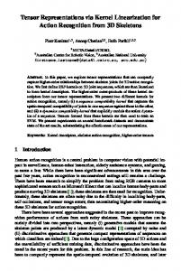
notably. It is worth noting that TAISL works even with only one source sample per category, which suggests that it can be applied for effective small-sample-size adaptation. Adaptation with noisy labels. Recent studies [41] demonstrate that tensor representations are inherently robust to noise. To further justify this in the context of DA, we randomly replace the source data with samples that have different labels. We gradually increase the percentage of noisy data Tnoisy from 0% to 20% and monitor the degradation of classification accuracy. As shown in Fig. 4(c), TAISL consistently demonstrates superior classification performance over other approaches. Convergence analysis and efficiency comparison. In this part, we empirically analyze the convergence behavior of TAISL. Fig. 4(d) shows the change of loss function as the iteration increases. It can be observed that the optimization generally converges in about 10 iterations. In addition, we also compare the efficiency of different approaches. The average evaluation time of each trial is reported. According to Table 1, the efficiency of TAISL is competitive too. TCA and LSSA are fast, because these two methods adopt kernel tricks to avoid high-dimensional computation implicitly. In general, learning a tensor subspace is faster than a vector subspace in the high-dimensional case.
Adaptation with limited source/target data. One of the important features of TAISL in practice is the small amount of training data required. In other words, one can characterize a domain, and thus adapt a pre-trained classifier, with very limited data. To demostrate this point, we evaluate the classification accuracy while varying the number of source/target data used for adaptation. The DA task of D → C is used. Concretely, we first fix the number of target data and, respectively, randomly choose from 1 to 8 source samples per category. In turn, we fix the number of source data to 8 per category and set the target samples per category to 2k , k = 0, 1, 2, ..., 7. Fig. 4(a)-(b) illustrate the results of different approaches. It can be observed that, our approach demonstrates very stable classification performance, while other comparing methods is sensitive to the number of source samples used. Meanwhile, the number of target data seems not to have much impact on the classification accuracy, because in general one prefers to transfer the source domain so that the target domain does not change
Recognition results. Quantitative results are listed in Table 2. It shows that our approach is on par with or outperforms other related and state-of-the-art methods in terms of both average accuracy and standard deviations. Note that conventional methods that directly adapt vector-form convolutional activations sometimes have a negative effect on the classification, even falling behind the baseline NA. The main reason perhaps is the inexact estimation of a large amount of parameters. For instance, in many subspacebased approaches, one needs to estimate a flattened subspace from the covariance matrix. Given a data matrix 7
90 90
80 80 70
Accuracy (%)
Accuracy (%)
70 60
Daum´e III TCA DIP SA LTSL LSSA CORAL NTSL TAISL
50 40 30 20
60 50
Daum´e III TCA DIP SA LTSL LSSA CORAL NTSL TAISL
40 30 20 10 0
10 0
1
2
3
4
5
6
7
8
10 0
9
10 1
Nsc
10 2
Ntc
(a)
(b)
90
A→C W→A D→C ImageNet→VOC2007
80
60
Loss
Accuracy (%)
70
50
Daum´e III TCA DIP SA LTSL LSSA CORAL NTSL TAISL
40 30 20 10 0 0
2
4
6
8
10
12
14
16
18
20
0
5
Tnoisy (%)
10
15
20
Iteration (d)
(c)
Figure 4: Adaptation on D→C with (a) varying number of source data per class Nsc , (b) a varying number of target data per class Ntc , and (c) noisy source labels. (d) Empirical convergence analysis of TAISL over several DA tasks. Daum´e III
TCA
GFK
DIP
SA
0.06
0.05
3.94
9.09
3.40
80
LTSL
LSSA
CORAL
NTSL
TAISL
70
12.34
0.59
14.81
0.16
0.92
90
Table 1: Average evaluation time (min) of each trial of different methods on A→C. (Matlab 2016a, OS: OS X 64-bit, CPU: Intel i5 2.9GHz, RAM: 8 GB)
NA NTSL TAISL
80 70 Accuracy (%)
Accuracy (%)
Method Time Method Time
60 50
NA NTSL TAISL
60 50 40 30
40
20
30
10 HOG
CONV (VGG-M) CONV (VGG-VD)
(a) A→C
A ∈ Rd×n with dimension d and n samples, its covariance matrix is estimated as AAT . Notice that rank(A) = rank(AAT ) = rank(AT A) ≤ min(d, n − 1). If d � n, the vector subspace will only be spanned by less than n eigenvectors. In addition, one also suffers from the problem of biased estimation [35] (large eigenvalues turn larger, small ones turn smaller) when d � n. Hence, such vector subspaces are unreliable. In contrast, our approach avoids this problem due to the mode-wise parameters estimation.
HOG
CONV (VGG-M) CONV (VGG-VD)
(b) W→A
Figure 5: Adaptation accuracy of three types of tensor representations on two DA tasks. a multi-label dataset, so many images contain multiple labels. Results are listed in Table 5. Due to the space limitation, we show only results of 10 categories (additional results are attached in the Supplementary). We observe that TAISL still demonstrates the best overall classification performance among comparing approaches. We also notice that NTSL and TAISL show comparable results. We conjecture that, since the target domain contains too many noisy labels, it will be hard to determine a global alignment that just matches class-level differences. As a result, the
5.3. Evaluation on the ImageNet–VOC2007 dataset Here we evaluate our approach under a more challenging dataset than OC10. As aforementioned, VOC2007 is 8
Method NA PCA Daum´e III TCA GFK DIP SA LTSL LSSA CORAL NTSL TAISL
A→C
C→A
A→D
D→A
A→W
W→A
C→D
D→C
C→W
W→C
D→W
W→D
MEAN
77.3(1.8) 36.7(3.0) 73.1(1.5) 56.7(4.5) 75.1(3.9) 59.8(5.7) 67.7(4.2) 70.2(2.4) 80.3(2.3) 77.6(1.2) 78.5(2.3) 80.1(1.4)
89.0(2.0) 57.7(5.2) 85.9(2.5) 78.1(6.1) 87.6(2.3) 84.8(4.3) 82.0(2.6) 87.5(2.8) 86.4(1.7) 80.3(1.9) 89.6(2.2) 90.0(1.9)
82.8(2.2) 23.5(8.1) 70.9(3.7) 59.9(6.7) 81.4(4.3) 52.2(8.1) 67.8(4.8) 77.7(4.6) 90.9(1.7) 64.3(2.9) 83.1(3.3) 85.1(2.2)
81.1(1.9) 50.2(4.8) 59.9(7.1) 61.2(4.2) 90.4(1.4) 76.4(3.7) 77.4(6.0) 69.2(4.5) 92.3(0.6) 74.2(2.2) 87.8(1.4) 87.6(2.1)
74.6(3.1) 18.6(6.2) 70.6(3.5) 55.5(6.4) 74.3(5.2) 45.5(9.1) 61.1(5.1) 66.7(4.6) 84.0(1.7) 61.2(2.4) 77.3(3.1) 77.9(2.6)
74.0(2.5) 51.2(6.0) 68.7(4.4) 68.3(4.1) 84.0(4.4) 69.3(6.9) 80.1(4.3) 66.6(5.7) 86.6(4.5) 69.1(2.6) 85.8(2.8) 85.6(3.5)
86.2(4.0) 29.9(7.8) 81.4(4.1) 74.3(5.2) 84.8(4.5) 82.8(7.7) 73.7(4.3) 82.3(4.1) 73.5(2.3) 62.1(3.0) 87.7(2.9) 90.6(1.9)
70.5(1.9) 51.0(3.3) 56.2(6.4) 51.9(2.2) 82.2(2.4) 61.9(6.3) 66.9(3.3) 60.8(3.1) 65.9(6.5) 72.0(1.7) 79.8(1.5) 84.0(1.0)
79.4(2.7) 26.4(6.7) 75.4(4.0) 69.0(6.6) 81.9(4.9) 73.5(4.9) 65.9(4.0) 75.3(4.2) 45.4(6.6) 63.8(3.1) 80.4(3.8) 85.3(3.1)
63.7(2.1) 51.6(3.6) 59.6(2.6) 54.7(3.8) 79.1(2.7) 65.2(4.5) 70.4(4.1) 59.1(4.4) 29.5(7.0) 66.6(2.2) 80.0(2.0) 82.6(2.2)
91.1(1.7) 49.5(4.2) 81.5(2.7) 89.8(2.2) 92.8(2.2) 90.9(2.3) 87.3(3.1) 86.0(2.9) 93.4(2.2) 89.6(1.6) 95.4(1.4) 95.9(1.0)
94.9(2.4) 50.8(7.0) 86.5(4.9) 90.6(3.2) 95.2(2.2) 94.1(3.1) 91.1(3.3) 90.0(3.8) 85.8(4.7) 82.8(2.8) 97.8(1.7) 97.7(1.5)
80.4 41.4 72.5 67.5 84.1 71.4 74.3 74.3 76.2 72.0 85.3 86.9
Table 2: Average multi-class recognition accuracy (%) on Office–Caltech10 dataset over 20 trials. The highest accuracy in each column is boldfaced, the second best is marked in red, and standard deviations are shown in parentheses. Method NA PCA Daum´e III TCA GFK DIP SA LTSL LSSA CORAL NTSL TAISL
aero 66.4(2.1) 28.9(5.8) 64.1(3.7) 43.2(9.8) 70.0(6.9) 69.8(5.5) 64.4(10.1) 56.9(10.4) 78.7(2.0) 71.4(3.3) 76.3(4.3) 76.4(5.1)
bird 65.6(4.0) 30.2(3.9) 59.7(7.4) 44.4(10.5) 74.6(3.8) 78.4(4.6) 69.3(5.4) 61.0(7.7) 79.7(1.2) 71.7(3.6) 71.0(3.9) 71.6(3.1)
bottle 29.5(2.1) 23.3(5.2) 26.6(3.3) 20.7(1.7) 32.5(4.4) 29.1(5.0) 34.4(4.6) 34.9(6.2) 38.4(4.6) 35.2(2.4) 35.7(3.7) 36.7(3.5)
cat 70.6(3.4) 44.9(4.5) 65.7(5.3) 56.7(8.2) 73.1(6.5) 75.9(3.7) 67.4(4.9) 70.8(8.8) 81.7(0.5) 72.0(4.3) 71.3(3.2) 72.0(2.1)
cow 30.3(8.0) 6.0(1.8) 26.9(8.5) 16.9(6.3) 28.9(5.3) 25.5(5.0) 18.4(6.6) 21.9(6.3) 29.5(1.9) 36.0(5.7) 34.7(9.8) 33.3(6.6)
table 35.7(5.5) 29.0(6.9) 30.0(5.4) 27.6(8.7) 48.3(10.4) 42.2(8.1) 36.9(12.8) 43.7(12.4) 33.7(3.4) 40.6(6.7) 49.8(10.4) 50.7(10.0)
mbike 47.0(8.0) 25.0(5.0) 40.5(6.6) 31.8(10.2) 58.3(4.8) 56.3(5.7) 53.7(10.9) 52.5(10.7) 56.3(9.3) 57.3(5.6) 59.7(10.2) 60.3(8.7)
person 69.3(2.9) 70.2(1.9) 68.5(2.5) 58.1(5.7) 75.8(3.6) 73.5(3.1) 68.9(2.4) 69.9(4.3) 51.2(2.0) 67.6(2.0) 72.0(4.6) 72.2(3.8)
sheep 44.9(6.9) 11.7(3.5) 37.7(7.4) 22.7(8.0) 52.5(4.8) 48.9(4.3) 31.4(10.2) 38.2(9.5) 32.5(10.6) 54.8(2.9) 53.4(6.0) 53.6(5.6)
tv 56.4(3.3) 29.0(6.6) 51.9(4.4) 33.6(10.2) 57.1(4.5) 59.4(5.2) 55.2(5.7) 54.0(7.5) 51.6(4.6) 56.9(3.6) 60.2(3.5) 60.4(3.5)
mAP 51.6 29.8 47.2 35.6 57.1 55.9 50.0 50.4 53.3 56.6 58.4 58.7
Table 3: Average precision (%) on ImageNet–VOC2007 dataset over 10 trials. The highest performance in each column is boldfaced, the second best is marked in red, and standard deviations are shown in parentheses. alignment may not work the way it should. In addition, according to Tables 2 and 5, LSSA shows superior accuracy than ours over several DA tasks/categories. It makes sense because LSSA works at different levels with further nonlinearity and samples reweighting. However, non-linearity is a double-edged sword. It can improve the accuracy in some situations, while sometimes it may not. For instance, the accuracy of LSSA drops significantly on the W→C task.
tal rule of domain-invariant feature representations for DA.
6. Conclusion Practical application of machine learning techniques often gives rise to situations where domain adaptation is required, either because acquiring the perfect training data is difficult, the domain shift is unpredictable, or simply because it is easier to re-use an existing model than to train a new one. This is particularly true for CNNs as the training time and data requirements are significant. The DA method proposed in this work is applicable in the case where a tensor representation naturally captures information that would be difficult to represent using vector arithmetic, but also benefits from the fact that it uses a lower-dimensional representation to achieve DA, and thus is less susceptible to noise. We have shown experimentally that it outperforms the state of the art, most interestingly for CNN DA, but is also much more efficient. In future work, discriminative information from source data may be employed for learning a more powerful invariant tensor subspace.
5.4. Evaluation with other tensor representations Finally, we evaluate other types of tensor representations to validate the generality of our approach. We do not limit the representation from deep learning features. Other shallow tensor features also can be adapted by our approach. Specifically, the improved HOG feature [9] and convolutional activations extracted from the CONV5 layer of VGG– M [4] model are further utilized and evaluated on two DA tasks from the OC10 dataset. Results are shown in Fig. 5. We notice that TAISL consistently improves the recognition accuracy with various tensor representations. In addition, a tendency shows that, the better feature representations are, the higher the baseline achieves, which implies a fundamen9
Appendix In this Appendix, we provide more details that are not included in the main text due to the page limitation. In particular, we supplement the following content on • how to implement the optimization of our approach efficiently; • how to perform spatial pooling normalization to convolutional activations; we only briefly mention this procedure in Section 5.1 of the main text; • detailed introduction regarding used datasets; • additional results evaluated on Office and ImageNet–VOC2007 datasets; • parameters sensitivity.
7. Towards efficient optimization In this section, we will reveal several important details towards efficient practical implementations. Note that Xs ∈ Rn1 ×...×nK ×Ns is a (K + 1)-mode tensor, the unfolding matrix X s(k) is of size nk × n\k Ns , where n\k = n1 · · · nk−1 nk+1 · · · nK . When computing Q(k) = X s(k) M T\k in Eq. (13), M T\k will be of size n\k Ns × n\k Ns , which is extremely large and consume a huge amount of memory to store. In fact, such a matrix even cannot be constructed in a general-purpose computer. To alleviate this, we choose to solve an equivalent optimization problem by reformulating Eq. (13) into its sum form as Ns X min kM (k) Qn(k) − Y n(k) k2F − λkM (k) X ns(k) k2F M (k) , (18) n=1 s.t. ∀k, M (k) M (k)T = I where ˆT Qn(k) = X ns(k) M \k ˆ T = M (K) ⊗ · · · ⊗ M (k+1) ⊗ M (k−1) ⊗ · · · ⊗ M (1) M \k
,
(19)
Y n(k) = Y (k) (:, :, n) (Y (k) has been reshaped into the size of nk × n\k × Ns ), and X ns(k) denotes the k-th mode unfolding matrix of Xsn . In following expressions, we denote Qn(k) , Y n(k) , and X ns(k) by Qn , Y n , and X n for short, respectively. By replacing M (k)T with P , we arrive at
min P
Ns X
kQTn P − Y Tn k2F − λkX Tn P k2F
n=1
.
(20)
T
s.t. ∀k, P P = I Considering that a standard solver needs the loss function F and its gradient ∂F/∂P as the input, we can compute them in the following way to speed up the optimization process. For the loss function F, we have F =
Ns X
kQTn P − Y Tn k2F − λkX Tn P k2F
n=1
=
Ns X
Ns h i h i X T r (QTn P − Y Tn )T (QTn P − Y Tn ) − λ T r (X Tn P )T (X Tn P )
n=1
=
Ns X
n=1
h
i
T r P T Qn QTn P − 2P T Qn Y Tn + Y n Y Tn − λ
Ns X
, (21) h i T r P T X n X Tn P
n=1
n=1
" T
= Tr P (
Ns X n=1
# Qn QTn )P
" T
− 2T r P (
Ns X
# Qn Y
T n)
n=1
+ Tr
"N s X n=1
10
# Y nY
T n
" T
− λT r P (
Ns X
n=1
# X n X Tn )P
where T r[·] denotes the trace of matrix. For the gradient ∂F/∂P , we have ∂F/∂P = 2
Ns X
Qn (QTn P − Y Tn ) − 2λ
n=1
= 2(
Ns X
Ns X
X n X Tn P
n=1
Qn QTn )P − 2
n=1
Ns X
Qn Y Tn − 2λ(
n=1
Ns X
.
(22)
X n X Tn )P
n=1
PNs T Notice that both F and ∂F/∂P share some components. As a consequence, we can precompute n=1 Qn Qn , P P PNs Ns Ns T T T n=1 X n X n before the M-step optimization instead of directly feeding the origin=1 Y n Y n , and n=1 Qn Y n , nal variables and iteratively looping over Ns samples inside the optimization. Such a kind of precomputation speeds up the optimization significantly.
8. Feature normalization with spatial pooling Since we allow the input image to be of arbitrary size, a normalization step need to perform to ensure the consistency of dimensionality. The idea of spatial pooling is similar to the spatial pyramid pooling in [14]. The difference is that we do not pool pyramidally and do not vectorize the pooled activations, in order to preserve the spatial information. Intuitively, Fig. 6 illustrates this process. More concretely, convolutional activations are first equally divided into Nbin bins along the spatial modes (Nbin = 16 in Fig. 6). Next, each bin with size of h × w is normalized to a s × s bin by max pooling. In our experiments, we set Nbin = 36 and s = 1.
9. Datasets and protocol details Office–Caltech10 dataset. As mentioned in the main text, [12] extends Office [26] dataset by adding another Caltech domain. They select 10 common categories from four domains, including Amazon, DSLR, web-cam, and Caltech. Amazon consists of images used in the online market, which shows the objects from a canonical viewpoint. DSLR contains images captured with a high-resolution digital camera. Images in web-cam are recorded using a low-end webcam. Caltech is similar to Amazon but with various viewpoint variations. The 10 categories include backpack, bike, calculator, headphones, keyboard, laptop computer, monitor, mouse, mug, and projector. Some images of four domains are shown in Fig. 7. Overall, we have about 2500 images and 12 domain adaptation problems. For each problem, we repeat the experiment 20 times. In each trail, we randomly select 20 images from each category for training if the domain is Amazon and Caltech, or 8 images if the domain is DSLR or web-cam. All images in the target domain are employed in the both adaptation and testing stages. The mean and standard deviation of multi-class accuracy are reported. Office dataset. Office dataset is developed by [26] and turns out to be a standard benchmark for the evaluation of domain adaptation. It consists of 31 categories and 3 domains, leading to 6 domain adaptation problems. Among these 31 categories, only 16 overlap with the categories contained in the 1000-category ImageNet 2012 dataset1 [16], so Office dataset is more challenging than its counterpart Office-Caltech10 dataset. We follow the same experimental protocol mentioned above to conduct the experiments, so in each task we have 620 images in all from the source domain. 1 The 16 overlapping categories are backpack, bike helmet, bottle, desk lamp, desk computer, file cabinet, keyboard, laptop computer, mobile phone, mouse, printer, projector, ring binder, ruler, speaker, and trash can.
Max Pooling
Spatial Pooling
h w
s s
Figure 6: Illustration of spatial pooling normalization. Any size of convolutional representations will be normalized to a fixed-size tensor. 11
Amazon
DSLR
web-cam
Caltech
Figure 7: Some images from Office–Caltech10 dataset. 4 categories of backpack, bike, headphone, and laptop computer are selected.
ImageNet
VOC2007
Figure 8: Some images from ImageNet-VOC2007 dataset. 5 categories of person, dog, motorbike, bicycle, and cat are presented. ImageNet–VOC2007 dataset. As described in the main text, ImageNet and VOC 2007 datasets are used to evaluate the domain adaptation performance from single-label to multi-label situation. The same 20 categories as the VOC 2007 dataset are chosen from original ImageNet dataset. These 20 categories are aeroplane, bicycle, bird, boat, bottle, bus, car, cat, chair, cow, dining table, dog, horse, motorbike, person, potted plant, sheep, sofa, train, and tv monitor. The 20-category ImageNet subset is adopted as the source domain, and the test subset of VOC2007 is employed as the target domain. Some images of two domains are illustrated in Fig. ??. Also, the similar experimental protocol mentioned above is used. The difference, however, is that we report the mean and standard deviation of average precision (AP) for each category, respectively.
10. Recognition results We compare against the same methods used in the main text, including the baseline no adaptation (NA), principal components analysis (PCA), transfer component analysis (TCA) [23], geodesic flow kernel (GFK) [12], domain-invariant projection (DIP) [2], subspace alignment (SA) [10], low-rank transfer subspace learning (LTSL) [29], landmarks selection subspace alignment (LSSA) [1], and correlation alignment (CORAL) [31]. Our approach is denoted by NTSL (the naive version) and TAISL. We also extract convolutional activations from the CONV5 3 layer of the VGG–VD–16 model [30]. We mark the feature as V CONV and T CONV for vectorized and tensor-form convolutional activations, respectively. The same parameters described in the main text are set to report the results. Office results. Results of the Office dataset are listed in Table 4. Similar to the tendency shown by the results of OfficeCaltech10 dataset in the main text, our approach outperforms or is on par with other comparing methods. It is interesting that sometimes NTSL even achieves better results than TAISL. We believe such results are sound, because a blind global adaptation cannot always achieve accuracy improvement. However, it is clear that learning an invariant tensor space works much better than learning a shared vector space. Furthermore, the joint learning effectively reduces the standard deviation and thus improves the stability of the adaptation. 12
Method
Feature
A→D
D→A
A→W
W→A
D→W
W→D
MEAN
NA
V CONV
53.8(2.3)
39.3(1.7)
47.7(1.7)
36.3(1.6)
77.4(1.7)
81.3(1.5)
56.0
PCA
V CONV
40.5(3.3)
38.2(2.6)
36.5(2.9)
37.8(2.9)
68.7(2.5)
70.5(2.6)
48.7
DAUME
V CONV
48.4(2.5)
35.2(1.5)
42.5(2.0)
33.6(1.8)
68.4(2.5)
74.2(2.4)
50.4
TCA
V CONV
30.3(4.5)
20.1(4.4)
27.0(3.1)
18.1(3.0)
51.1(3.2)
53.0(3.2)
33.3
GFK
V CONV
DIP SA
V CONV
47.4(4.7) 36.8(4.5)
36.2(2.9) 13.8(1.8)
41.5(3.5) 29.6(5.0)
33.4(2.6) 17.8(2.6)
75.3(1.6) 77.4(1.8)
78.0(2.4) 81.5(2.0)
51.9 42.8
V CONV
28.6(3.5)
37.1(2.1)
29.0(2.1)
34.9(2.9)
75.1(2.4)
75.1(2.7)
46.6
LTSL
V CONV
32.0(5.5)
28.6(1.6)
24.2(3.7)
27.1(2.0)
60.9(4.0)
73.9(3.3)
41.1
LSSA
V CONV
56.6(2.0)
45.6(1.6)
52.2(1.6)
40.7(2.0)
73.0(2.1)
63.5(3.8)
55.3
CORAL
V CONV
39.9(1.7)
42.7(0.9)
39.7(1.7)
40.7(1.0)
82.0(1.3)
79.5(1.4)
54.1
NTSL
T CONV
56.1(2.4)
45.7(1.5)
50.8(2.3)
42.6(2.2)
84.4(1.6)
88.2(1.4)
61.3
TAISL
T CONV
56.4(2.4)
45.9(1.1)
50.7(2.0)
43.2(1.7)
84.5(1.4)
88.5(1.2)
61.5
Table 4: Average multi-class recognition accuracy (%) on Office dataset over 20 trials. The highest accuracy in each column is boldfaced, the second best is marked in red, and standard deviations are shown in parentheses.
Feature Mode
Spatial Mode
90
90
90
88
80
85
Sensitivity of λ
86
70 80
84
70 65
Accuracy
Accuracy
Accuracy
60 75
50 40
82 80 78
30
76 60
20
NTSL TAISL
55
NTSL TAISL
10 0
50 1
2
3
4
5
ds
6
10 0
10 1
10 2
df
74 72 70 10 -10
10 -5
10 0
λ
Figure 9: Sensitivity of tensor subspace dimensionality and weight coefficient λ on the DA task of W→C. ImageNet–VOC2007 results. Table 5 shows the complete results on ImageNet–VOC2007 dataset (only partial results are presented in the main text due to the page limitation). Our approach achieves the best mean accuracy in 4 and the second best in 6 out of 20 categories. In general, when noisy labels exist in the target domain, our approach demonstrates a stable improvement in accuracy. Moreover, compared to the baseline NTSL, the standard deviation is generally reduced, which means aligning the source domain to the target not only promotes the classification accuracy but also improves the stability of tensor space.
11. Parameters Sensitivity Here we investigate the sensitivity of 3 parameters involved in our approach. Specifically, they are the spatial mode dimensionality ds (d1 and d2 in the main text, we assume d1 = d2 = ds ), the feature mode dimensionality df (d3 in the main text), and the weight coefficient λ. We monitor how the classification accuracy changes when these parameters vary. At each time, only one parameter is allowed to change. By default, ds = 6, df = 128, and λ = 1e−5 . A DA task of W→C from the Office-Caltech10 dataset is chosen. Results are illustrated by Fig. 9. According to Fig. 9, we can make the following observations: • In general, there exhibits a tendency for increased ds to increased classification accuracy, which implies that the adaptation can benefit from extra spatial information. This is why we preserve the original spatial mode as it is. • As per the feature mode dimensionality df , a dramatic growth appears when df increases from 1 to 16. However, the 13
aero
bike
bird
boat
bottle
bus
car
cat
chair
cow
NA
VOC 2007 test V CONV
66.4(2.1)
65.3(2.9)
65.6(4.0)
56.1(9.0)
29.5(2.1)
51.2(3.4)
70.9(4.5)
70.6(3.4)
19.3(2.0)
30.3(8.0)
PCA
V CONV
28.9(5.8)
25.3(7.2)
30.2(3.9)
14.0(4.8)
23.3(5.2)
15.6(6.3)
41.5(7.5)
44.9(4.5)
11.2(0.9)
6.0(1.8)
Daum´e III
V CONV
64.1(3.7)
60.4(4.2)
59.7(7.4)
53.5(7.8)
26.6(3.3)
49.0(5.1)
66.3(5.1)
65.7(5.3)
18.6(3.5)
26.9(8.5)
TCA
V CONV
43.2(9.8)
46.0(17.0)
44.4(10.5)
25.3(13.0)
20.7(1.7)
30.4(7.7)
59.5(8.6)
56.7(8.2)
17.1(3.0)
16.9(6.3)
GFK
V CONV
70.0(6.9)
66.0(7.6)
74.6(3.8)
40.7(11.8)
32.5(4.4)
55.0(6.9)
71.3(5.2)
73.1(6.5)
16.3(3.6)
28.9(5.3)
DIP
V CONV
69.8(5.5)
65.8(7.2)
78.4(4.6)
34.2(9.1)
29.1(5.0)
54.4(7.3)
75.7(3.9)
75.9(3.7)
20.1(4.6)
25.5(5.0)
SA
V CONV
64.4(10.1)
54.4(9.3)
69.3(5.4)
50.8(12.7)
34.4(4.6)
50.8(6.5)
64.3(9.5)
67.4(4.9)
11.2(1.9)
18.4(6.6)
LTSL
V CONV
56.9(10.4)
59.8(6.3)
61.0(7.7)
50.6(15.6)
34.9(6.2)
50.9(9.6)
66.9(3.6)
70.8(8.8)
11.4(1.5)
21.9(6.3)
LSSA
V CONV
78.7(2.0)
71.8(1.5)
79.7(1.2)
18.5(2.0)
38.4(4.6)
64.1(3.2)
69.4(2.2)
81.7(0.5)
57.2(2.4)
29.5(1.9)
CORAL
V CONV
71.4(3.3)
63.3(4.3)
71.7(3.6)
58.6(9.5)
35.2(2.4)
61.9(3.6)
62.7(7.1)
72.0(4.3)
18.7(2.7)
36.0(5.7)
NTSL
T CONV
76.3(4.3)
61.6(5.5)
71.0(3.9)
65.9(8.3)
35.7(3.7)
56.1(7.1)
70.1(4.8)
71.3(3.2)
16.6(2.6)
34.7(9.8)
TAISL
T CONV
76.4(5.1)
62.3(4.8)
71.6(3.1)
64.9(7.7)
36.7(3.5)
57.0(6.6)
71.2(4.3)
72.0(2.1)
15.7(2.9)
33.3(6.6)
table
dog
horse
mbike
person
plant
sheep
sofa
train
tv
mAP
NA
V CONV
35.7(5.5)
47.9(6.4)
35.5(11.4)
47.0(8.0)
69.3(2.9)
25.6(3.9)
44.9(6.9)
46.9(5.3)
71.8(4.4)
56.4(3.3)
50.3
PCA
V CONV
29.0(6.9)
32.5(4.6)
23.2(6.2)
25.0(5.0)
70.2(1.9)
9.3(4.3)
11.7(3.5)
16.2(2.8)
29.0(6.7)
29.0(6.6)
25.8
Daum´e III
V CONV
30.0(5.4)
43.6(6.9)
28.3(8.7)
40.5(6.6)
68.5(2.5)
23.6(3.5)
37.7(7.4)
44.5(5.6)
67.6(5.4)
51.9(4.4)
46.4
TCA
V CONV
27.6(8.7)
43.2(7.6)
29.0(14.6)
31.8(10.2)
58.1(5.7)
11.6(4.5)
22.7(8.0)
24.0(9.4)
52.3(8.9)
33.6(10.2)
34.7
GFK
V CONV
48.3(10.4)
56.7(7.4)
59.2(16.7)
58.3(4.8)
75.8(3.6)
15.2(4.6)
52.5(4.8)
44.7(6.0)
79.9(4.9)
57.1(4.5)
53.8
DIP
V CONV
42.2(8.1)
53.7(5.4)
64.7(7.1)
56.3(5.7)
73.5(3.1)
14.7(4.2)
48.9(4.3)
39.8(10.0)
80.5(5.6)
59.4(5.2)
53.1
SA
V CONV
36.9(12.8)
54.2(5.7)
39.5(15.5)
53.7(10.9)
68.9(2.4)
20.9(6.7)
31.4(10.2)
29.3(6.1)
73.5(5.2)
55.2(5.7)
47.4
LTSL
V CONV
43.7(12.4)
55.4(7.4)
53.4(13.1)
52.5(10.7)
69.9(4.3)
18.8(8.2)
38.2(9.5)
28.9(13.2)
67.1(9.9)
54.0(7.5)
48.3
LSSA
V CONV
33.7(3.4)
56.9(2.5)
41.1(5.4)
56.3(9.3)
51.2(2.0)
15.3(5.7)
32.5(10.6)
43.4(8.4)
81.1(1.4)
51.6(4.6)
52.6
CORAL
V CONV
40.6(6.7)
53.8(5.3)
34.8(6.8)
57.3(5.6)
67.6(2.0)
24.2(1.5)
54.8(2.9)
47.7(6.2)
71.7(3.5)
56.9(3.6)
53.0
NTSL
T CONV
49.8(10.4)
58.3(5.1)
40.9(12.9)
59.7(10.2)
72.0(4.6)
25.0(4.5)
53.4(6.0)
49.8(4.6)
75.3(3.6)
60.2(3.5)
55.2
TAISL
T CONV
50.7(10.0)
57.6(3.8)
39.0(14.0)
60.3(8.7)
72.2(3.8)
26.6(5.4)
53.6(5.6)
49.8(5.6)
74.2(4.9)
60.4(3.5)
55.3
Table 5: Average precision (%) on ImageNet-VOC2007 dataset over 10 trials. The highest AP in each column is boldfaced, the second best is marked in red, and standard deviations are shown in parentheses. classification accuracy starts to level off when df exceeds 16. Such results make sense, because when the feature dimensionality is relatively small, the discriminative power of feature representations cannot be guaranteed. Overall, our approach demonstrates stable classification performance over a wide range of feature mode dimensionality. • Only a slight fluctuation occurs when λ varies between 1e−9 and 1e1 . The classification accuracy is virtually insensitive to the weight coefficient λ. This is another good property of our approach. Acknowledgments. This work was supported in part by the National High-tech R&D Program of China (863 Program) under Grant 2015AA015904 and in part by the National Natural Science Foundation of China under Grant 61502187.
References [1] R. Aljundi, R. Emonet, D. Muselet, and M. Sebban. Landmarks-based kernelized subspace alignment for unsupervised domain adaptation. In Proc. IEEE Conference on Computer Vision and Pattern Recognition (CVPR), pages 56–63, 2015. [2] M. Baktashmotlagh, M. T. Harandi, B. C. Lovell, and M. Salzmann. Unsupervised domain adaptation by domain invariant projection. In Proc. IEEE International Conference on Computer Vision (ICCV), pages 769–776, 2013. [3] S. Ben-David, J. Blitzer, K. Crammer, F. Pereira, et al. Analysis of representations for domain adaptation. In Advances in Neural Information Processing Systems (NIPS), volume 19, page 137, 2007. [4] K. Chatfield, K. Simonyan, A. Vedaldi, and A. Zisserman. Return of the devil in the details: Delving deep into convolutional nets. In Proc. British Machine Vision Conference (BMVC), 2014. [5] W.-S. Chu, F. De La Torre, and J. F. Cohn. Selective transfer machine for personalized facial action unit detection. In Proc. IEEE Conference on Computer Vision and Pattern Recognition (CVPR), June 2013. [6] H. Daum´e III. Frustratingly easy domain adaptation. In Proc. Association for Computational Linguistics (ACL), 2007.
14
[7] J. Deng, W. Dong, R. Socher, L.-J. Li, K. Li, and L. Fei-Fei. Imagenet: A large-scale hierarchical image database. In Proc. IEEE Conference on Computer Vision and Pattern Recognition (CVPR), pages 248–255, 2009. [8] M. Everingham, L. Van Gool, C. K. Williams, J. Winn, and A. Zisserman. The pascal visual object classes (VOC) challenge. International Journal of Computer Vision, 88(2):303–338, 2010. [9] P. F. Felzenszwalb, R. B. Girshick, D. McAllester, and D. Ramanan. Object detection with discriminatively trained part-based models. IEEE Transactions on Pattern Analysis and Machine Intelligence, 32(9):1627–1645, 2010. [10] B. Fernando, A. Habrard, M. Sebban, and T. Tuytelaars. Unsupervised visual domain adaptation using subspace alignment. In Proc. IEEE International Conference on Computer Vision (ICCV), pages 2960–2967, 2013. [11] Y. Ganin and V. Lempitsky. Unsupervised domain adaptation by backpropagation. In Proc. International Conference on Machine Learning (ICML), pages 1180–1189, 2015. [12] B. Gong, Y. Shi, F. Sha, and K. Grauman. Geodesic flow kernel for unsupervised domain adaptation. In Proc. IEEE Conference on Computer Vision and Pattern Recognition (CVPR), pages 2066–2073, 2012. [13] R. Gopalan, R. Li, and R. Chellappa. Domain adaptation for object recognition: An unsupervised approach. In Proc. IEEE International Conference on Computer Vision (ICCV), pages 999–1006, 2011. [14] K. He, X. Zhang, S. Ren, and J. Sun. Spatial pyramid pooling in deep convolutional networks for visual recognition. IEEE Transactions on Pattern Analysis and Machine Intelligence, 37(9):1904–1916, 2015. [15] K. He, X. Zhang, S. Ren, and J. Sun. Deep residual learning for image recognition. In Proc. IEEE Conference on Computer Vision and Pattern Recognition (CVPR), 2016. [16] J. Hoffman, E. Tzeng, J. Donahue, Y. Jia, K. Saenko, and T. Darrell. One-shot adaptation of supervised deep convolutional models. In Proc. International Conference on Learning Representations Workshops (ICLRW), 2013. [17] T. K. Kim and R. Cipolla. Canonical correlation analysis of video volume tensors for action categorization and detection. IEEE Transactions on Pattern Analysis and Machine Intelligence, 31(8):1415–1428, Aug 2009. [18] T. G. Kolda and B. W. Bader. Tensor decompositions and applications. SIAM review, 51(3):455–500, 2009. [19] A. Krizhevsky, I. Sutskever, and G. E. Hinton. Imagenet classification with deep convolutional neural networks. In Advances in Neural Information Processing Systems (NIPS), pages 1097–1105, 2012. [20] X. Li, W. Hu, Z. Zhang, X. Zhang, and G. Luo. Robust visual tracking based on incremental tensor subspace learning. In Proc. IEEE International Conference on Computer Vision (ICCV), pages 1–8. IEEE, 2007. [21] J. Long, E. Shelhamer, and T. Darrell. Fully convolutional networks for semantic segmentation. In 2015 IEEE Conference on Computer Vision and Pattern Recognition (CVPR), pages 3431–3440, June 2015. [22] H. Lu, Z. Cao, Y. Xiao, and Y. Zhu. Two-dimensional subspace alignment for convolutional activations adaptation. Pattern Recognition, 71:320–336, 2017. [23] S. J. Pan, I. W. Tsang, J. T. Kwok, and Q. Yang. Domain adaptation via transfer component analysis. IEEE Transactions on Neural Networks, 22(2):199–210, Feb 2011. [24] V. M. Patel, R. Gopalan, R. Li, and R. Chellappa. Visual domain adaptation: A survey of recent advances. IEEE Signal Processing Magazine, 32(3):53–69, 2015. [25] S. Ren, K. He, R. Girshick, and J. Sun. Faster R-CNN: Towards real-time object detection with region proposal networks. In Proc. Advances in Neural Information Processing Systems (NIPS), pages 91–99, 2015. [26] K. Saenko, B. Kulis, M. Fritz, and T. Darrell. Adapting visual category models to new domains. In Proc. European Conference on Computer Vision (ECCV), pages 213–226, 2010. [27] O. Sener, H. O. Song, A. Saxena, and S. Savarese. Learning transferrable representations for unsupervised domain adaptation. In Advances in Neural Information Processing Systems (NIPS), pages 2110–2118, 2016. [28] G. Shakhnarovich and B. Moghaddam. Face recognition in subspaces. In Handbook of Face Recognition, pages 19–49. Springer, 2011. [29] M. Shao, D. Kit, and Y. Fu. Generalized transfer subspace learning through low-rank constraint. International Journal of Computer Vision, 109(1-2):74–93, 2014. [30] K. Simonyan and A. Zisserman. Very deep convolutional networks for large-scale image recognition. CoRR, abs/1409.1556, 2014. [31] B. Sun, J. Feng, and K. Saenko. Return of frustratingly easy domain adaptation. In Proc. AAAI Conference on Artificial Intelligence, 2016. [32] L. Van der Maaten and G. Hinton. Visualizing data using t-SNE. Journal of Machine Learning Research, 9(2579–2605):85, 2008. [33] M. A. O. Vasilescu and D. Terzopoulos. Multilinear analysis of image ensembles: Tensorfaces. In Proc. European Conference on Computer Vision (ECCV), pages 447–460. Springer, 2002. [34] M. A. O. Vasilescu and D. Terzopoulos. Multilinear subspace analysis of image ensembles. In Proc. IEEE Conference on Computer Vision and Pattern Recognition (CVPR), volume 2, pages II–93. IEEE, 2003. [35] L. Wang, J. Zhang, L. Zhou, C. Tang, and W. Li. Beyond covariance: Feature representation with nonlinear kernel matrices. In Proc. IEEE International Conference on Computer Vision (ICCV), pages 4570–4578, 2015.
15
[36] Y. Wen, K. Zhang, Z. Li, and Y. Qiao. A discriminative feature learning approach for deep face recognition. In Proc. European Conference on Computer Vision (ECCV), pages 499–515. Springer, 2016. [37] Z. Wen and W. Yin. A feasible method for optimization with orthogonality constraints. Mathematical Programming, 142(1-2):397– 434, 2013. [38] J. Yosinski, J. Clune, Y. Bengio, and H. Lipson. How transferable are features in deep neural networks? In Advances in Neural Information Processing Systems (NIPS), pages 3320–3328, 2014. [39] L. Zhang, W. Wei, C. Tian, F. Li, and Y. Zhang. Exploring structured sparsity by a reweighted laplace prior for hyperspectral compressive sensing. IEEE Transactions on Image Processing, 25(10):4974–4988, 2016. [40] L. Zhang, W. Wei, Y. Zhang, C. Shen, A. van den Hengel, and Q. Shi. Dictionary learning for promoting structured sparsity in hyperspectral compressive sensing. IEEE Transactions on Geoscience and Remote Sensing, 54(12):7223–7235, 2016. [41] Q. Zhao, L. Zhang, and A. Cichocki. Bayesian CP factorization of incomplete tensors with automatic rank determination. IEEE Transactions on Pattern Analysis and Machine Intelligence, 37(9):1751–1763, Sept 2015.
16