In press, The American Statistician
Where’s Waldo: Visualizing Collinearity Diagnostics Michael Friendly∗
Ernest Kwan
Abstract Collinearity diagnostics are widely used, but the typical tabular output used in almost all software makes it hard to tell what to look for and how to understand the results. We describe a simple improvement to the standard tabular display, a graphic rendition of the salient information as a “tableplot,” and graphic displays designed to make the information in these diagnostic methods more readily understandable. In addition, we propose a visualization of the contributions of the predictors to collinearity through a collinearity biplot, which is simultaneously a biplot of the smallest dimensions of the cor−1 relation matrix of the predictors, RXX , and the largest dimensions of RXX , on which the standard collinearity diagnostics are based. Key words: condition indices, collinearity biplot, diagnostic plots, effect ordering, multiple regression, tableplot, variance inflation
1
Introduction Q: (Collinearity diagnostics and remedies): ”Some of my collinearity diagnostics have large values, or small values, or whatever they’re not supposed to have. Is this bad? If so, what can we do about it?” from: http://www.sociology.ohio-state.edu/people/ptv/faq/ collinearity.htm
Problems in estimation in multiple regression models that arise from influential observations and high correlations among the predictors were first described in a comprehensive way in Belsley, Kuh, and Welsch’s (1980) Regression Diagnostics: Identifying Influential Data and Sources of Collinearity. This book would prove to be a highly influential point on the landscape of diagnostic methods for regression, but not always one of high leverage, at least in graphical methods for visualizing and understanding collinearity diagnostics. Later, David Belsley wrote A guide to using the collinearity diagnostics (Belsley, 1991b), that seemed to promise a solution for visualizing these diagnostics. For context, it is worth quoting the abstract in total: ∗ Michael Friendly is Professor, Psychology Department, York University, Toronto, ON, M3J 1P3 Canada, E-mail:
[email protected]. Ernest Kwan is Assistant Professor, Sprott School of Business, Carleton University, E-mail: ernest
[email protected]. This work is supported by Grant 8150 from the National Sciences and Engineering Research Council of Canada. We are grateful to John Fox for comments on an initial draft and to the referees for helping us to clarify the presentation.
1
The description of the collinearity diagnostics as presented in Belsley, Kuh, and Welsch’s, Regression Diagnostics: Identifying Influential Data and Sources of Collinearity, is principally formal, leaving it to the user to implement the diagnostics and learn to digest and interpret the diagnostic results. This paper is designed to overcome this shortcoming by describing the different graphical displays that can be used to present the diagnostic information and, more importantly, by providing the detailed guidance needed to promote the beginning user into an experienced diagnostician and to aid those who wish to incorporate or automate the collinearity diagnostics into a guided-computer environment. Alas, the “graphical displays” suggested were just tables– of eigenvalues, condition numbers and coefficient variance proportions associated with the collinearity diagnostics. There is no doubt that Belsley’s suggested tabular displays have contributed to the widespread implementation and use of these diagnostics. Yes, as the initial quote for this introduction indicates, users are often uncertain about how to interpret these tabular displays. To make the point of this paper more graphic, we liken the analyst’s task in understanding collinearity diagnostics to that of the reader of Martin Hansford’s successful series of books, Where’s Waldo (titled Where’s Wally in the UK, Wo ist Walter in Germany, etc.). These consist of a series of full-page illustrations of hundreds of people and things and a few Waldos— a character wearing a red and white striped shirt and hat, glasses, and carrying a walking stick or other paraphernalia. Waldo was never disguised, yet the complex arrangement of misleading visual cues in the pictures made him very hard to find. Collinearity diagnostics often provide a similar puzzle. The plan of this paper is as follows: We first describe a simple example that illustrates the current state of the art for the presentation of collinearity diagnostics. Section 2 summarizes the standard collinearity diagnostics in relation to the classical linear regression model, y = Xβ + ǫ. In Section 3 we suggest some simple improvements to the typical tabular displays and a graphic rendering called a “tableplot” to make these diagnostics easier to read and understand. Section 4 describes some graphic displays based on the the biplot (Gabriel, 1971) that helps interpret the information in collinearity diagnostics. It is also important to say here what this paper does not address: collinearity in regression models is a large topic, and the answer to the last question in the initial quote, If so, what can we do about it? would take this article too far afield. The methods described below do provide a means to see what is potentially harmful, whether large or small and thus, answers the question Is this bad? More importantly, the graphic displays related to these questions can often say why something about the data is good or bad.
1.1
Example: Cars data
As a leading example, we use the Cars dataset from the 1983 ASA Data Exposition (http://stat-computing. org/dataexpo/1983.html) prepared by Ernesto Ramos and David Donoho. This dataset contains 406 observations on the following seven variables: MPG (miles per gallon), Cylinder (# cylinders), Engine (engine displacement, cu. inches), Horse (horsepower), Weight (vehicle weight, lbs.), Accel (time to accelerate from 0 to 60 mph, in sec.), and Year (model year, modulo 100). An additional categorical variable identifies the region of origin (American, European, Japanese), not analyzed here. For this data, the natural questions concern how well MPG can be explained by the other variables. Collinearity diagnostics are not part of the standard output of any widely-used statistical software; they must be explicitly requested by using options (SAS), menu choices (SPSS) or other packages (R: car, perturb). 2
As explained in the next section, the principal collinearity diagnostics include: (a) variance inflation factors, (b) condition indices, and (c) coefficient variance proportions. To obtain this output in SAS, one can use the following syntax, using the options VIF and COLLINOINT. proc reg data = cars; model mpg = weight year engine horse accel cylinder / vif collinoint; run; Another option, COLLIN, produces collinearity diagnostics that include the intercept. But these are useless unless the intercept has a real interpretation and the origin on the regressors is contained within the predictor space, as explained in Section 2.2. See Fox (1997, p. 351) and the commentary surrounding Belsley (1984) for discussion of this issue. We generally prefer the intercept-adjusted diagnostics, but the choice is not material to the methods presented here. The model specified above fits very well, with an R2 = 0.81; however, the t-tests for parameters shown in Table 1 indicates that only two predictors— Weight and Year are significant. Table 1 also shows the variance inflation factors. By the rules-of-thumb described below, four predictors— Weight, Engine, Horse and Cylinder have potentially serious problems of collinearity, or at least cause for concern. The condition indices and coefficient variance proportions are given in Table 2. As we describe below, we might consider the last two rows to show evidence of collinearity. However, the information presented here hardly gives rise to a clear understanding. Table 1: Cars data: parameter estimates and variance inflation factors Variable DF Parameter Standard t Value Pr > |t| Variance Estimate Error Inflation Intercept 1 −14.63175 4.88451 −3.00 0.0029 0 Weight 1 −0.00678 0.00067704 −10.02 100 is a sign of potential disaster in estimation. Coefficient variance proportions : Large VIFs indicate variables that are involved in some nearly collinear relations, but they don’t indicate which other variable(s) each is involved with. For this purpose, Belsley et al. (1980) and Belsley (1991a) proposed calculation of the proportions of variance of each variable associated with each principal component as a decomposition of the coefficient variance for each dimension. These may be expressed (Fox, 1984, §3.1.3) as pjk =
2 Vjk V IFj λk
(5)
Note that for orthogonal regressors, all condition indices κk = 1 and the matrix of coefficient variance proportions, P = (pjk ) = I. Thus, Belsley (1991a,b) recommended that the sources of collinearity be diagnosed (a) only for those components with large κk , and (b) for those components for which pjk is large (say, pjk ≥ 0.5) on two or more variables.
3 Improved tabular displays: How many Waldos? The standard tabular display of condition indices and variance proportions in Table 2 suffers mainly from the fact that the most important information is disguised by being embedded in a sea of mostly irrelevant numbers, arranged by inadvertent design to make the user’s task harder. One could easily nominate this design as a Where’s Waldo for tabular display. The first problem is that the table is sorted by decreasing eigenvalues. This would otherwise be typical and appropriate for eigenvalue displays, but for collinearity diagnostics, it hides Waldo among the bottom rows. It is more useful to sort by decreasing condition numbers. A second problem is that the variance proportions corresponding to small condition numbers are totally irrelevant to problems of collinearity. Including them, perhaps out of a desire for completeness, would otherwise be useful, but here it helps Waldo avoid detection. For the purpose for which these tables are designed, it is better simply to suppress the rows corresponding to low condition indices. In
5
this article we adopt the practice of showing one more row than the number of condition indices greater than 10 in tables, but there are even better practices. Software designers who are troubled by incompleteness can always arrange to make the numbers we would suppress perceptually less important, e.g., smaller in size or closer to background in texture or shading, as in Table 3. A simple version of this is to use a ’fuzz’ value, e.g., fuzz=0.5 such that all variance proportions < fuzz are blanked out, or replaced by a place holder (’.’). For example, the colldiag function in the R package perturb (Hendrickx, 2008) has a print method that supports a fuzz argument. The third problem is that, even for those rows (large condition numbers) we want to see, the typical displayed output offers Waldo further places to hide among numbers printed to too many decimals. Do we really care that the variance proportion for Engine on component 5 is 0.00006088? For the large condition numbers, we should only be concerned with the variables that have large variable proportions associated with those linear combinations of the predictors. For the Cars data, we need only look at the rows corresponding to the highest condition indices. Any sharp cutoff for the coefficient variance proportions to display (e.g., pjk ≥ 0.5) runs into difficulties with borderline values, so in Table 3, we highlight the information that should capture attention by (a) removing all decimals and (b) distinguishing values ≥ 0.5 by font size and style; other visual attributes could also be used. From this, it is easily seen that there are two Waldos in this picture. The largest condition index corresponds to a near linear dependency involving Engine size and number of cylinders; the second largest involves weight and horsepower, with a smaller contribution of acceleration. Both of these have clear interpretations in terms of these variables on automobiles: engine size is directly related to number of cylinders and, orthogonal to that dimension, there is a relation connecting weight to horsepower. Table 3: Cars data: Revised condition indices and variance proportions display. Variance proportions > 0.5 are highlighted. Condition Proportion of Variation (×100) Number Index Eigenvalue Weight Year Engine Horse Accel Cylinder 6 10.96 0.03545 18 1 98 4 1 56 5 8.43 0.05987 71 7 0 66 49 11
3.1
Tableplots
Table 2 and even the collinearity-targeted version, Table 3, illustrate how difficult it is to display quantitative information in tables so that what is important to see— patterns, trends, differences, or special circumstances— are made directly visually apparent to the viewer. Tukey (1990) referred to this property as interoccularity: the message hits you between the eyes. A tableplot is a semi-graphic display designed to overcome these difficulties, developed by Ernest Kwan (2008a). The essential idea is to display the numeric information in a table supplemented by symbols whose size is proportional to the cell value, and whose other visual attributes (shape, color fill, background fill, etc.) can be used to encode additional information essential to direct visual understanding. The method is far more general than described here and illustrated in the context of collinearity diagnostics. See Kwan (2008b) for some illustrations of the use for factor analysis models.
6
CondIndex
Weight
Year
Engine
Horse
Accel
Cylinder
#6 10.96
18
1
98
4
1
56
8.43
71
7
0
66
49
11
5.67
9
1
1
29
6
32
2.5
1
5
0
0
42
1
2.26
1
86
0
0
0
0
1
0
1
0
1
1
0
#5
#4
#3
#2
#1
Figure 1: Tableplot of condition indices and variance proportions for the Cars data. In column 1, the square symbols are scaled relative to a maximum condition index of 30. In the remaining columns, variance proportions (×100) are shown as circles scaled relative to a maximum of 100. Figure 1 is an example of one tableplot display design for collinearity diagnostics. All the essential numbers in Table 2 are shown, but encoded in such a way as to make their interpretation more direct. The condition indices are shown by the area of the white squares in column 1. In this example these are scaled so that a condition index of 30 corresponds to a square that fills the cell. The background color of the cells in this column indicate a reading of the severity of the condition index, κk . In this example, green (”OK”) indicates κk < 5, yellow (”warning”) indicates 5 ≤ κk < 10 and red (”danger”) indicates κk ≥ 10. The remaining columns show the collinearity variance proportions, 100 × pjk , with circles scaled relative to a maximum of 100, and with color fill (white, pink, red) distinguishing the ranges { 0–20, 20–50, 50–100}. The details of the particular assignments of colors and ranges to the condition indices and variance proportions are surely debatable, but the main point here is that Figure 1 succeeds where Table 2 does not and Table 3 only gains by hiding irrelevant information.
7
4 Graphical displays: biplots As we have seen, the collinearity diagnostics are all functions of the eigenvalues and eigenvectors of the correlation matrix of the predictors in the regression model, or alternatively, the SVD of the X matrix in the linear model (excluding the constant). The standard biplot (Gabriel, 1971, Gower and Hand, 1996) can be regarded as a multivariate analog of a scatterplot, obtained by projecting a multivariate sample into a low-dimensional space (typically of 2 or 3 dimensions) accounting for the greatest variance in the data. With the symmetric (PCA) scaling used here, this is equivalent to a plot of principal component ˜ of predictors for the observations (shown as points or case labels), scores of the mean-centered matrix X together with principal component coefficients for the variables (shown as vectors) in the same 2D (or 3D) space. The standard biplot, of the first two dimensions, corresponding to the largest eigenvalues of RXX is shown in Figure 2. This is useful for visualizing the principal variation of the observations in the space of the predictors. It can be seen in Figure 2 that the main dimension of variation among the automobile models is in terms of engine size and power; acceleration time is also strongly related to Dimension 1, though of course inversely. The second dimension (accounting for an additional 13.8% of predictor variance) is largely determined by model year. In these plots: (a) The variable vectors have their origin at the mean on each variable, and point in the direction of positive deviations from the mean on each variable. (b) The angles between variable vectors portray the correlations between them, in the sense that the cosine of the angle between any two variable vectors approximates the correlation between those variables (in the reduced space). (c) Similarly, the angles between each variable vector and the biplot axes approximate the correlation between them. (d) Because the predictors were scaled to unit length, the relative length of each variable vector indicates the proportion of variance for that variable represented in the low-rank approximation. (e) The orthogonal projections of the observation points on the variable vectors show approximately the value of each observation on each variable. (f) By construction, the observations, shown as principal component scores are uncorrelated; But the standard biplot is less useful for visualizing the relations among the predictors that lead to nearly collinear relations. Instead, biplots of the smallest dimensions show these relations directly, and can show other features of the data as well, such as outliers and leverage points.
4.1
Visualizing variance proportions
As with the tabular display of variance proportions, Waldo is hiding in the dimensions associated with the smallest eigenvalues (largest condition indices). As well, it turns out that outliers in the predictor space— high leverage observations— can often be seen as observations far from the centroid in the space of the smallest principal components. Figure 3 shows the biplot of the Cars data for the smallest two dimensions— what we can call the collinearity biplot. The projections of the variable vectors on the Dimension 5 and Dimension 6 axes are proportional to their variance proportions in Table 2. The relative lengths of these variable vectors can be considered to indicate the extent to which each variable contributes to collinearity for these two near-singular dimensions. Thus, we see that (as in Table 3) Dimension 6 is largely determined by Engine size, with a substantial relation to Cylinder. Dimension 5 has its’ strongest relations to Weight and Horse. In the reduced tabular display, Table 3, we low-lighted all variance proportions < 0.5, but this is unnecessary in the graphical representation.
8
year
Dimension 2 (13.76%)
1.0
0.5
373 396 297 398 395 375 306 372 298 369 300 296 295 374 308 293 401 381 324 406 376 403 382 405 377367402 299 294 397 371 378379 380 399 370 273 349 391 336 239 258 240 385388 400 389347 386 390 291 292 366 237 387 360 335 259 230 232231 305 394 368 393 384 323404 257 270 392 348 365 238 307 289 260 341 268288 364 346 322 272229 334 355354 350 358 356 264 269 363321 359 361 326 331 261265 266 327 198 220 357 271 352 333 351 196 285 195 353 221 164 315 343 267 167 222 216 328 197223 235 332 339345 262 236 166 165 330 318 314 329 290 325 234 283233 319 317 313 320 208 304 316 340 342 147 145 280279282 207 311 337 219209 168 210 111 146 148 98102103 310309 263 284 169 312 112 200 202 171 170 249 302 303 281 162 278 252 199 301 275 201 113 173 174 144 99 114 274 277 163218 217276 254255287 161 242 124 244 101 100 184 93 286 160 142 123 256243 96 95 75 141 78 250 177172 215 224 253 227 76 77104 71 143 245 225 251 8297 246 182 136 52 226 9472 73132 247 204 228 70 241248 192 83 203 5150 81129 133 190214 193 191 135 47 80 186 187 178 106 213 194181 74 48 46 206212 205 176 105 108 185 179 32 188 49 9 180 211 109107 33 34 6 87 115 175 189 140 14 131 12 138 183 158157 1319 15 149 121 10 2 139153 137 117 151 128 156 16 155 43 42 154 44 159 150 45 120 1 4 116 118 86 5655 130 17 53 110152 53 122 127 126 67 68 125 18 84 85 41 6988 89 65 90 87119 66 92 22 23 5491 11 2431 79 37 6459 40 63 57 38 2758 36 61 6029 62 28 26 21 30 25
weight cylinder engine
accel
horse
0.0
20
-0.5 -1.0
-0.5
0.0
0.5
1.0
Dimension 1 (71.39%)
Figure 2: Standard biplot of the Cars data, showing the first two dimensions. The observations are labeled with their case numbers and colored according to region of origin. The right half of the plot consists almost entirely of US cars (blue). Moreover, there is one observation, #20, that stands out as an outlier in predictor space, far from the centroid. It turns out that this vehicle, a Buick Estate wagon, is an early-year (1970) American behemoth, with an 8-cylinder, 455 cu. in, 225 horse-power engine, and able to go from 0 to 60 mph in 10 sec. (Its MPG is only slightly under-predicted from the regression model, however.) This and other high-leverage observations may be seen in other graphical displays; but it is useful to know here that they will often also be quite noticeable in what we propose here as the collinearity biplot. The web page of supplementary materials for this article (Section 5.2) shows a robust outlier-detection QQ plot and an influence plot of these data for comparison with more well-known methods.
4.2
Visualizing condition indices
The condition indices are defined q in terms of the ratios λ1 /λk (on a square root scale). It is common to refer to the maximum of these, λ1 /λp as the condition number for the entire system, giving the worst near-singularity for the entire model. A related visualization, that potentially provides more information than just the numerical condition indices can be seen in biplots of Dimension 1 vs. Dimension k, where, typically only the k corresponding to the smallest eigenvalues are of interest. To visualize the relative size of λk to λ1 it is useful to overlay this plot with a data ellipse for the component scores. Figure 4 shows the condition number biplot for the Cars data, where the condition number can be approximately seen as the ratio of the horizontal to the vertical dimensions of the data ellipse. As the
9
0.5
engine
20
0.4 0.3 Dimension 6 (0.58%)
x
7
x
0.2
x x x x x x x x xx x x x x x xx x x x x x x xxx x x xx x xx xxxx xx x x xx x x xx x xx x x x x xxxx x x xxx x x x x x x x x xx x x x xx x x x xx x xx xx xx x xxxxxxx xxxx xxx x x xxxx x x x xx xxxx x xxxxxxxxxxxx xx xxxxxxx x x x x x x x x xxx x xxxxxx xxxxxxx x xx xx xxx x x x x x x x x x x x x x xxx x x x x xxxxx xxxxxxxxxxxx xx xxxxxxxx xxxxxx xxxx xx x x x x x x x xx x x xx xx xxxxxx xxx x xx xxx x x xxx xx x x x xxx xx x xx xx xx xx xx x xx x x x xx xx x xx x xx x xx x xx xx x x x x xx x x x x xx x x x xx x x x x x x x x xx xx xx x x x x x x
103
x x
0.1
x
9
x
x
x
year accel
x
0.0 -0.1
weight -0.2
124
horse
32
x x x
x
xx x
-0.3
x cylinder x
34 33
x x
-0.4 -0.5 -0.4 -0.3 -0.2 -0.1
0.0
0.1
0.2
0.3
0.4
0.5
0.6
0.7
0.8
Dimension 5 (0.98%)
Figure 3: Collinearity biplot of the Cars data, showing the last two dimensions. The projections of the variable vectors on the coordinate axes are proportional to their variance proportions. To reduce graphic clutter, only the eight most outlying observations in predictor space are identified by case labels. An extreme outlier (case #20) appears in the upper right corner. numerical values of the condition indices in Table 2 also indicate, ill-conditioning in this example is not particularly severe. In general, however, the relative lengths of the variable vectors approximately indicate those variables that contribute to ill-conditioning. The observations can also be interpreted in this display in relation to their projections on the variable vectors. Case 20, the main high-leverage point is seen as having high projections on Dimension 1, which in this view is seen as the four variables with high VIFs: Engine, Horse, Weight, Cylinder. The observations that contribute to large condition indices are those with large projections on the smallest component, Dimension 6.
5 Other examples 5.1
Biomass data
Rawlings (1988, Table 13.1) described analyses of a data set concerned with the determination of soil characteristics influencing the aerial biomass production of a marsh grass, Spartina alterniflora in the Cape Fear estuary of North Carolina. The soil characteristics consisted of 14 physical and chemical properties, measured at nine sites (three locations × three vegetation types), with five samples per site, giving n = 45 observations. The data were collected as part of a Ph.D. dissertation by Richard Linthurst.
10
Dimension 6 (0.58%)
0.5
20
x x x xx x x x xx x x x xx x x x x xx xx xxx x xx x x x x xxxxxx xx xx x x x x x x x x x x xx xxx x x x xx x xxx x xx x x x xxx x x x x xx x xxxxx xx xxxx xx xxx x x x x x xx xxx xxx xx x xxx x x xxxxxxxxxxxxxxxxx xxxxxxxxxxxxxx xxxxxxxxxx x xxx x xx x x x x x xx x x x x xxxxxx x xx x xx x xxx x x xxxxxxxxxxxxxxxxxxxxxx x x x xx x x x xx xx x xx x x x xxxx x xxxxxxxxxx x x x x xx xxx xxx x xx xxx x x x xx x xxxxxxxxx xxx x xx x x x x xx x x x x x xx x x x x x x x x x xx x x xxxxx x xx x x xx x x x x x x x x x xx xx x x x x x x x x x x x x x x x x
accel
0.0
97 103
x
x
engine
xx
x x
year
x
124
32
3334
horse weight cylinder
-0.5 -1.0
-0.5
0.0
0.5
1.0
Dimension 1 (71.39%)
Figure 4: Condition number biplot of the Cars data, showing the first and last dimensions, with a 68% data ellipse for the component scores. The square root of the ratio of the horizontal and vertical axes of the ellipse portrays the condition number. The quantitative predictors (i.e., excluding location and type) were: H2S: free sulfide; sal: salinity; Eh7: redox potential at pH 7; pH: soil pH; buf: buffer acidity at pH 6.6; and concentrations of the following chemical elements and compounds— P: phosphorus; K: potassium; Ca: calcium; Mg: magnesium; Na: sodium; Mn: manganese; Zn: zinc; Cu: copper, NH4: ammonium. It should be noted that if the goal of the study was simply to describe biomass for the given timeframe and locations, collinearity would be less of an issue. But here, the emphasis in analysis focuses on identifying the “important” variable determinants of biomass. The model with all 14 quantitative predictors fits very well indeed, with an R2 = .81. However, the parameter estimates and their standard errors shown in Table 4 indicate that only two variables, K and Cu, have significant t statistics, all of the others being quite small in absolute value. For comparison, a stepwise selection analysis using 0.10 as the significance level to enter and remove variables selected the four-variable model consisting of pH, Mg, Ca and Cu (in that order), giving R2 = 0.75; other selection methods were equally inconsistent and perplexing in their possible biological interpretations. Such results are a clear sign-post of collinearity. We see from Table 4 that many of the VIFs are quite large, with six of them (pH, buf, Ca, Mg, Na and Zn) exceeding 10. How many Waldos are hiding here? The condition indices and variance proportions for the full model are shown, in our preferred form, in Table 5, where, according to our rule of thumb, 1+#(Condition Index> 10), we include the 4 rows with condition indices > 7. Following Belsley’s (1991a) rules of thumb, it is only useful to interpret those entries (a) for which the condition indices are large and (b) where two or more variables have large portions of their variance associated with a near singularity. Accordingly, we see that there are two Waldos contributing to collinearity: the smallest dimension (#14), consisting of the variables pH, buf, and Ca, and the next smallest (#13), consisting of Mg and Zn. The first of these is readily interpreted as indicating that soil pH is highly determined by buffer acidity and calcium concentration. Alternatively, Figure 5 shows a tableplot of the largest 10 condition indices and associated variance
11
Table 4: Linthall data: Parameter estimates and variance inflation factors Variable
DF
Intercept H2S sal Eh7 pH buf P K Ca Mg Na Mn Zn Cu NH4
1 1 1 1 1 1 1 1 1 1 1 1 1 1 1
Parameter Estimate 2909.93 0.42900 −23.980 2.5532 242.528 −6.902 −1.702 −1.047 −0.1161 −0.2802 0.00445 −1.679 −18.79 345.16 −2.705
Standard Error 3412.90 2.9979 26.170 2.0124 334.173 123.821 2.640 0.482 0.1256 0.2744 0.02472 5.373 21.780 112.078 3.238
t Value
Pr > |t|
VIF
0.85 0.14 −0.92 1.27 0.73 −0.06 −0.64 −2.17 −0.92 −1.02 0.18 −0.31 −0.86 3.08 −0.84
0.401 0.887 0.367 0.214 0.474 0.956 0.524 0.038 0.363 0.315 0.858 0.757 0.395 0.004 0.410
0 3.02 3.39 1.98 62.08 34.43 1.90 7.37 16.66 23.76 10.35 6.18 11.63 4.83 8.38
Table 5: Linthall data: Condition indices and variance proportions (×100). Variance proportions > 0.4 are highlighted. # 14 13 12 11
Cond Index 22.78 12.84 10.43 7.53
Eigen value 0.0095 0.0298 0.0453 0.0869
H2S
sal
Eh7
22 0 0 19
25 9 16 3
3 2 3 0
pH 95
buf 70
0 4 0
12 13 4
P
K
1 8 5 1
8 28 0 7
Ca 60
Mg
Na
Mn
16
1 16 18
67
21 25 28 5
34 16 2 14
15 1
Zn
Cu
NH4
2
4 0
17 21 24 2
45 9 32
43 9
proportions, using the same assignments of colors to ranges as described for Figure 1. Among the top three rows shaded red for the condition index, the contributions of the variables to the smallest dimensions is more readily seen than in tabular form (Table 5). The standard biplot (Figure 6) shows the main variation of the predictors on the two largest dimensions in relation to the observations; here, these two dimensions account for 62% of the variation in the 14-dimensional predictor space. As before, we can interpret the relative lengths of the variable vectors as the proportion of each variable’s variance shown in this 2D projection, and the (cosines of) the angles between the variable vectors as the approximation of their correlation shown in this view. Based on this evidence it is tempting to conclude, as did Rawlings (1988, p. 366) that there are two clusters of highly related variables that account for collinearity: Dimension 1, having strong associations with five variables (pH, Ca, Zn, buf, NH4), and Dimension 2, whose largest associations are with the variables K, Na and Mg. This conclusion is wrong! The standard biplot does convey useful information, but is misleading for the purpose of diagnosing collinearity because we are only seeing the projection into the 2D predictor space of largest variation and inferring, indirectly, the restricted variation in the small dimensions where Waldo usually hides. In the principal component analysis (or SVD) on which the biplot is based, the smallest four dimensions 12
CondIdx H2S sal #14
Eh7
pH
buf
P
K
Ca
Mg
Na
Mn
Zn
Cu NH4
22.78
22
25
3
95
70
1
8
60
16
21
34
2
4
17
12.84
0
9
2
0
12
8
28
1
67
25
16
45
0
21
10.43
0
16
3
4
13
5
0
16
15
28
2
9
43
24
7.53
19
3
0
0
4
1
7
18
1
5
14
32
9
2
5.87
20
11
2
0
0
0
29
0
0
13
15
0
2
13
5.45
6
5
16
0
0
2
26
1
0
0
1
10
18
13
3.6
0
1
13
0
0
22
0
1
0
5
12
1
4
1
3.57
8
11
12
0
0
16
0
0
0
1
1
0
17
5
3.14
12
0
36
0
0
0
0
2
0
0
3
0
0
3
2.67
0
11
2
0
0
43
0
0
0
1
0
0
0
0
#13 #12 #11 #10 #9 #8 #7 #6 #5
Figure 5: Tableplot of the 10 largest condition indices and variance proportions for the Linthall data. In column 1, the symbols are scaled relative to a maximum condition index of 30. In the remaining columns, variance proportions (×100) are scaled relative to a maximum of 100. (shown in Table 5) account for 1.22% of the variation in predictor space. Figure 7 shows the collinear−1 ity biplot for the smallest two dimensions of RXX , or equivalently, the largest dimensions of RXX , comprising only 0.28% of predictor variation. Again, this graph provides a more complete visualization of the information related to collinearity than is summarized in Table 5, if we remember to interpret only the long variable vectors in this plot and their projections on the horizontal and vertical axes. Variables pH, buf, and Ca to a smaller degree stand out on dimension 14, while Mg and Zn stand out on dimension 13. The contributions of the other variables and the observations to these nearly singular dimensions would give the analyst more information to decide on an effective strategy for dealing with collinearity.
5.2
Further examples and software
The data and scripts, for SAS and R, for these examples and others, will be available at www.math. yorku.ca/SCS/viscollin, where links for biplot and tableplot software will also be found.
6 Discussion As we have seen, the standard collinearity diagnostics— variance inflation factors, condition indices, and the variance proportions associated with each eigenvalue of RXX — do provide useful and relatively complete information about the degree of collinearity, the number of distinct near singularities, and the variables contributing to each. However, the typical tabular form in which this information is provided to the user is perverse— it conceals, rather than highlights, what is important to understand.
13
1.5
Mg
K Na Cu
1
1.0 92
Dimension 2 (26.39%)
Eh7
10 6
7 3
8
4
0.5
34 31
5
33
Zn
35 32 40
H2S sal
3938
36
45 44
0.0
37
42 43
pH
buf NH4
16 25
24
12 14
-0.5
27 28
Ca
13 41
20
21 23 17
11
19
26
P 22
Mn
15 18
29 30
-1.0 -1.5
-1.0
-0.5
0.0
0.5
1.0
1.5
Dimension 1 (35.17%)
Figure 6: Standard biplot of the Linthurst data, showing the first two dimensions. The point labels refer to case numbers, which are colored according to the location of the site. We have illustrated some simple modifications to the usual tabular displays designed to make it easier to see the number of Waldos in the picture and the variables involved in each. The re-ordered and reduced forms of these tables are examples of a general principle of effect ordering for data display (Friendly and Kwan, 2003) that translates here as “in tables and graphs, make the important information most visually apparent.” Tableplots take this several steps further to highlight what is important to be seen directly to the eye. The collinearity biplot, showing the smallest dimensions, does this too, but also provides a more complete visualization of the relations among the predictors and the observations in the space where Waldo usually hides.
References Belsley, D. A. (1984). Demeaning conditioning diagnostics through centering. The American Statistician, 38(2), 73–77. [with discussion, 78–93]. Belsley, D. A. (1991a). Conditioning Diagnostics: Collinearity and Weak Data in Regression. New York, NY: Wiley.
14
0.5
pH
0.4
Dimension 14 (0.07%)
buf
6
0.3
14 39
0.2
43 37
25
22
Na
0.1 33
Zn
0.0
13 21
28
NH4 40
20
42 17
15
-0.1
sal 1
K
9
32
Mn
29
36 12
2 16
41 45
30 Eh7 Cu 34 27 H2S 3
38 24
35 1126
31
8 44
4
Mg
10
7
23
-0.2
5
P
Ca
19
18
-0.3 -0.4
-0.3
-0.2
-0.1
0.0
0.1
0.2
0.3
0.4
0.5
0.6
Dimension 13 (0.21%)
Figure 7: Collinearity biplot of the Linthurst data, showing the last two dimensions Belsley, D. A. (1991b). A guide to using the collinearity diagnostics. Computer Science in Economics and Management, 4, 33–50. Belsley, D. A., Kuh, E., and Welsch, R. E. (1980). Regression Diagnostics: Identifying Influential Data and Sources of Collinearity. New York: John Wiley and Sons. Fox, J. (1984). Linear Statistical Models and Related Methods. New York: John Wiley and Sons. Fox, J. (1997). Applied Regression Analysis, Linear Models, and Related Methods. Thousand Oaks, CA: Sage Publications. Friendly, M. and Kwan, E. (2003). Effect ordering for data displays. Computational Statistics and Data Analysis, 43(4), 509–539. Gabriel, K. R. (1971). The biplot graphic display of matrices with application to principal components analysis. Biometrics, 58(3), 453–467. Gower, J. C. and Hand, D. J. (1996). Biplots. London: Chapman & Hall. Hendrickx, J. (2008). perturb: Tools for evaluating collinearity. R package version 2.03. Kwan, E. (2008a). Improving Factor Analysis in Psychology: Innovations Based on the Null Hypothesis Significance Testing Controversy. Unpublished doctoral dissertation, York University, Toronto, ON. Kwan, E. (2008b). Tableplot: A new display for factor analysis. (in preparation). 15
Marquandt, D. W. (1970). Generalized inverses, ridge regression, biased linear estimation, and nonlinear estimation. Technometrics, 12, 591–612. Rawlings, J. O. (1988). Applied Regression Analysis: A Research Tool. Pacific Grove, CA: Brooks/Cole Advanced Books. Tukey, J. W. (1990). Data-based graphics: Visual display in the decades to come. Statistical Science, 5(3), 327–339.
16