Paper accepted for presentation at 2003 IEEE Bologna PowerTech Conference, June 23-26, Bologna, Italy
Wind Power Forecasting using Fuzzy Neural Networks Enhanced with On-line Prediction Risk Assessment. P. Pinson and G. N. Kariniotakis. Member IEEE. Absfrad-The paper presents an advanced wind forecasting system that uses on-line SCAnA measurements, as well as numerical weather predictions (NWP) as input, to predict the power production of wind park8 48 hours ahead. The prediction system integrates models based on adaptive fuzzy-neural networks configured either for short-term (1-10 hours) or longterm (1-48 hours) forecasting. The paper presents detailed oneyear evaluation results ofthe models on the case study oflreland, where the output of several wind farms is predicted using HIRLAMmeteorological forecasts as input A method for the online estimation of confidence intervals of the forecasts is developed together with an appropriate index for assessing online the risk due to the inaccuracy of the numerical weather predictions. Index Term-Wind power, short-term forecasting, numerical weather predictions, on-line software, adaptive fuzzy-neural networks, confidenceintervals, prediction risk
N
I.
INTRODUCTION
OWADAYS, wind park installations in Europe exceed 23 GW, while the motivated by the Kyoto Protocol targets of the E.U. for 12% energy demand covered by renewables by year 2010, are translated to 21% electricity generation by renewables. To achieve these targets, wind power in the Member States should arise up to 45-60 GW. Such a large-scale integration of wind power emerges the development of appropriate tools to assist the wind farm operators on their management task. Short-term forecasts of the wind farms production, up to 48 hours ahead, are necessary for a secure and economic largescale wind power integration. Wind power prediction tools are useful for end-users such as Independent Power Producers, Transmission and Distribution System Operators (TSODSO), Energy Service Providers (ESP) etc. In a liberalised electricity market environmenf such tools enhance the competitiveness of wind power, since they reduce the penalties resulting from the wind resource intermittence. Reduced operational and financial risk for the wind farm developers is a motivating factor for undertaking investments on wind farms. Hence, accurate wind power prediction tools contribute indirectly to the increase of the installed wind power capacity. Wind power forecasting is a far from trivial problem. Wind speed is a non-stationary process both in the mean and variance. Wind power is nonlinear w.1.t. speed with a major difficulty in the area of cut-off speed, where prediction intervals can extend from maximum to zero wind power. Part of this work WBS supported by the European Commission in the frame of the contracts N’ ERK5CT1999-00019 and ENK5CT-200200665. G. N. Kariniotakis and P. Plnson are with the Center of Energy Studies of Eeole des Mines de Paris (e-mail:
[email protected],
[email protected]).
0-7803-7967-5/03/$17.0002003 IEEE
Among the difficulties, one should add the error of numerical weather forecasts, which are often used as input to the models. Often, no adequate information is available online by a data acquisition system (SCADA)to assess the actual operational status of the wind farm (i.e. how many turbines are in operation). The available on-line data can be detailed (i.e. power, speed of each wind turbine) or not (i.e. only total power available). In some situations there is complete lack of data and information from neighbor wind farms has to be assessed. Research on wind power forecasting is actively pursued by several research centres in Europe. Actually there are two main state-of-the-art approaches; one based on physical or deterministic modelling and a second one based on statistical or timeseries modelling. The “physical” approach for wind power forecasting is based on a detailed description of the wind park site (orography, roughness, obstacles), the wind turbines (hub height, power curve, thrust curve) and the layout of the wind plant. In [lo-121, wind power forecasting platforms based on physical methods are described. The main input is numerical weather predictions Oywp). Model output statistics are developed to account for systematic errors. Weather predictions are however updated only a limited number of times per day by meteorological services. For this reason, the performance of these models is often satisfactory for rather longer (% hours ahead) than short-term horizons. The alternative ‘‘time series”, or statistical, approach includes typical linear models (ARMA, ARX etc) and nonlinear ones (i.e. neural networks, conditional parametric models, etc). These models aim to predict the future by “capturing” temporal and spatial dependencies in the data [15]. The input to these models can be on-line SCADA data and numerical weather predictions (NWF’). For look-ahead times more than -10 hours (mentioned hereafter as “longterm”), NWPs are indispensable for an acceptable performance, since they represent weather dynamics that cannot be modelled using only recent on-line data. For shorter horizons, up to -10 hours ahead (mentioned hereafter as “short-term”), time series models can be based exclusively on recent measurements; however even in this case, NWPs as explanatory input improves results. It is noted that the threshold of 10 hours is mentioned as an example rather than a rule, since it depends on the characteristics of a specific wind profile. The model presented in this paper belongs to the time series approach. In previous work of the authors, linear autoregressive models, radial basis functions, wavelet networks, feed forward and recurrent neural networks [ 6 ] ,[7], and finally adaptive fuzzy-neural network models were
compared for the task of short-term predidion. F u v y neural networks, originally used here for wind forecasting, were found to outperform the other approaches in both masks of short-term and long-term wind prediction 191. 11. THEPREDICTIONMODULE.
Adaptive fuzzy-neural networks (F-NN) are applied here for both short-term and long-term wind power prediction. The adaptivity property stands for the capacity of the model to fine-tune its parameters during on-line operation. This is an important requirement for a non-stationary process like wind speed or power. Adaptivity of the model compensates changes in the environment of the application that may happen during the lifetime of a wind farm. Such changes can be changes in the number of wind turbines (extension of the wind farm, maintenance or availability of the machines that is usually not available through SCADA), in the performance of the wind turbines due to aging, changes in the surrounding of the wind park (i.e. vegetation), or changes in the configuration of the model used to produce the NWPs. The core F-NN model is generic and can be trained on appropriate input depending on the final use, which can be either short-term or long-term prediction.
E. Models based on meteorological information. For “long-term” horizons up to 24-48 hours ahead, it is necessary to include numerical weather predictions (NWP) as explanatory input to the model in order to have an acceptable performance. NWPs include usually wind speed, direction and temperature at 10 m, as well as at several altitude levels defined by atmospheric pressure. NWPs can be provided for the geographical coordinates of the wind farm or for a grid of four points surrounding the farm. In the second case, the spatial resolution of the NWP model is of primary importance. Meteorological models with high resolution are often more accurate hut require high computation time to produce forecasts, and as a consequence, they do not update frequently their output (i.e. 1-4 times per day). In contrast, forecasts from low-resolutionNWP models are more kquently available. The developed forecasting tool is able to operate with input from different NWP systems. In the frame of this work it was tested and gave satisfactory results with input from the SKIRON system for the case of Crete, and also from MRLAM for the case of Ireland. SKIRONforecasts were provided for a grid of 15x15 km (System B in &. I), while HIRLAM predictions we provided at the level of the wind farm (System A in F Z ~/)..
A . Short-term models. Short-term models receive historic values of wind power as input, as well as explanatory data, such as wind speed and direction, to predict wind power. The general form of a simple model with input only past values of power is:
i++I)=f(p(t)p(t-ll.. &m)) The generic fuzzy-neural function A.) is described in Section 111. Multi-step ahead forecasts are generated using the model in an iterative way. Le., in order to produoe a forecast for r+2, the forecast for t+l is fed back as input to the model. This approach presents the drawback that does not permit to iterate explanatory input, since no forecasts can be available for such quantities. To handle this problem, models using the look-ahead time k as an input variable can be considered. An alternative approach is to develop multi-output models, 01 to tune a different model for each time-step. The implementation of this approach is complex and requires high development effort, which can be prohibitive in case of a large number of wind farms. The short-term models based on fuzzy-neural networks can be useful for horizons up to -10 hours, They are found to outperform Persistence up to 20% according to the time-step 17-91. Persistence is a simple approach used as reference to evaluate the performance of advanced models. It assumes that the ‘’wind in the future will be the same as the wind now”. Short-term predictions are adequate for small applications, for which NWPs are not available, e.g. in the case of islands. In larger systems, timeseries models based on meteorological information, as the one presented below, outperform shortterm models (improvement up to 40% w.r.t. persistence for horizons up to IO hours).
Fig. I . General scheme ofthe “~ong-lerm”prediction model with evlmples
o f w o confrgualiomofNWP sysrems used as input (SKt~on! HiRLAMJ.
The developed model receives on-line data as well as NWPs as input to predict the wind farms production for the next 48 hours. These forecasts are updated every hour based on the most recent wind power measurements. Wind power data are necessary for the on-line updating procedure, independently if they are used or not as input variables to the model. The updating procedure permits mainly a good performance of the model for the first hours (i.e. 1-6 hours) of the considered horizon. Model configurations that do not update their forecasts based on recent wind power data were found to perform worse than persistence in look-ahead times up to 6 hours ahead. Finally, the consideration of on-line information, other than wind power (i.e. wind speed or direction), was not found to contribute in the accuracy of the results. The general scheme of the model is shown in Fig. 1, The aim of the prediction model is to capture the relations between input (meteorological information, on-line data) and output (future total wind park power). Such mapping includes the following implicit relations:
Temporal correlations between past and future data of the process (autoregressive aspect of the model). Conversion of wind speed (meteorological predictions) from the height or the atmospheric level they are given to the huh height of the wind turbines. Spatial projection of the meteorological wind speed forecasts from the NWP grid points (e.g. 15x15 km) to the level of the wind f m (“downscaling”). Correction of the wind park output for factors affecting the total production (i.e. a m y effects, effect of wind direction etc). The advantage - of a model such as the fuzzy neural network model, compared to models based on the “physical” approach, is that it permits to avoid all the above intermediate modeling steps. Moreover, its adaptive mode can compensate situations like the ones explained in the previous Section. 111.
property of the model, especially in the case of a nonstationary process such as wind generation. Fuzzy sets in the premises are modeled here using Gaussian functions:
Fic. 2. Reprerentofion offizzy wind speedr ‘‘*e&“is n linguistic variable with with three terms “slow”,“medium”,and ‘yast”represented arfizzy the membershipfunctions shown in the Figure.
In the case of a linear function in the consequence, the model may be Written analytically as following:
MODELDEVELOPMENT AND GENERALIZATION.
A . General description of thefuzry-neural network model
The fuuy model can he expressed in the form of rules of the type: “IF x_ is A THEN y is B“ where x, y are linguistic variables and A , B are fuzzy sets. In the case of time-series prediction rules may have the form:
R : IF
I, is
A,, and
.._,and
xn is A,
THEN y = g ( x , ,..., x,,)
where: xi,. ..,xn
A ,,...,A, Y
are real-valued variables representing input variables of the system defined in the universes of discourseXl, ..& respectively. are fuzzy sets. is variable of the consequence whose value is inferred. In the specific problem it represents future wind power &f+l)i(t+2) is a function that implies the value of y when x,, ...J” satisfy the premise. The functiong(.) in the consequent part of the rules may be a linear or a non-linear one or even a constant. In the case of a linear function the fuzzy rule-base takes the form:
,...).
g(.)
R‘:
IF x, is A: ,..., and xn is A:
R”:
IF
x, is A;
,..., and
x. is Anm
l”y ’ = p A + p : x I + ...+pix.
THEN y - =p,” +p; x,+...+p.“xn
Each rule gives an estimation of the output y j according to the conditions defined by the fuzzy sets in the premises. In the context of timeseries prediction, each variable x, in the premise corresponds to a past value of the process (i.e. power: P(t), P(t-1) ...), or past values of explanatory input (i.e. wind speed WS(f), WS(t-I)...) or meteorological forecasts (WS,,,(t+I), WS,(t+Z), . ..). A linear function in the consequence is indeed an ARX (autoregressive with exogenous variables) model. It is clear that with the above definitions, the rule-base consists of an ensemble of “local” models. Local modeling is a desired
E. Learning and Generalization. Model building is characterized by two phases: (i) optimization of the model architecture and (ii) tuning of the model internal parameters (learning). These two phases are driven by the requirement for good “generalization”. Generalization is the capacity of the model to perform well when it predicts new data (data not used during the two phases of model development). It is a primary requirement for the on-line use of a model. The tuning of the model parameters is performed taking into account [6]: * Learning rules based on stochastic gradient for tuning the parameters a, b , p of the model. * Learning rules are appropriately developed to minimize simultaneously prediction error and the Information content of the model (max entropy). This acts as a self regularization process that permits to avoid overfitting of the data. Simulated annealing is performed for controlling the evolution of the learning process through appropriate adaptation of the learning rate. Early-stopping is applied to the learning process is early-to avoid overfitting. * Cross-validation is applied to terminate learning. For this purpose, a subset of the data (validation set) is reserved. The cross-validation criterion is expressed as a weighted function of the performance of the model over the whole prediction horizon. By this way, generalization is optimized for multi-step ahead prediction. The above process permits to tune optimally a model with a specific architecture. The architecture of a model is defined by the types of input variables and the number of fuzzy sets associated to each one. For each type of measured data it is needed to decide the number of past values to be used as
input. When W P s are considered (“past values” have no sense), it is necessary to select the relevant information (forecasts of wind speed, direction, etc) for the model. This selection procedure, which is also similar to other types o f models like neural networks, is a time consuming one due to the infinite number of combinations that can be tested. Often it is performed by trial-and-error, where several candidate configurations are tested. It is noted that the evaluation of each candidate model requires carrying out the above-described learning process. In this work, the trial-and-error has been replaced by a fully automated process for model architecture optimization. The constrained nonlinear simplex (“Complex”) optimization algorithm is used for this purpose. The algorithm has been modified for handling both discrete and continuous decision variables. The optimization process is based on the evaluation of the surface o f the generalization function (defined as the performance of a model on the validation set) using a complex of points. Each point corresponds to a candidate model. The computational cost is high due to the necessity of the algorithm to tune each candidate model. However, in global, the automatic nature of the process permits to save considerable engineering time compared to the trial-and-error. Clmn.nl#rsb” cntsnon
HllbrnWnd*p..a (IOrn,
‘T
,, ...........
~1
WrndPW‘l .......... ........... .,......... ~~
consequent part. Parsimony in the selection of input is critical to avoid overfitting from overparametrized models. Fig. 3 shows an example of a run of the Complex algorithm. 115 candidate models are totally examined. The input selection is performed among past values of wind power and HlRLAM wind speed, direction and temperature forecasts. The upper left figure shows the evolution of the Complex objective function. Each point in the figure corresponds to the “generalization” performance of a candidate model on the validation set. The rest of Figures show the number of fuzzy sets associated by the algorithm to each input type of data. When the number of fuzzy sets for all variables is either one or zero then a single “rule” is obtained. The premise has no significance and the model corresponds to a simple linear function of the input variables. This limit case corresponds to the ARX class of models. Consequently, the optimization process can indeed exclude the use of a nonlinear fuzzy model and lead to a classical linear one. In this way, a selection between linear and nonlinear models is performed. 1V. UNCERTAINTYOF THE WIND POWER PREDICTIONS.
Spot predictions of the wind f m production for the next 48 hours is a primary requirement for end-users. However, for
““““1
nlmm D m o ” 110 m1 ............... ............. .............. .......... ~
Fiz. 3. Evolution of the olgwithmfor the model architecture oplimlronon
An alternative genetic algorithm approach did not present any advantages with respect to the simpler “Complex” algorithm. Genetic algorithms appeared to be less parsimonious w.r.t the number of models they need to test in order to converge compared to the Complex algorithm Each decision variable in Complex represents the number of fuzzy sets associated to each type of input data. In the special case, when the algorithm converges to zero-number of fuzzy sets for a specific type of data, then this input is excluded from the model as non-significant. By this way the algorithm performs input selection. When the number of fuuy sets is converging to one, then the variable does not participate in the premises, but appears only in the function of the
an optimal management of the wind power production it is necessary to provide end-users with appropriate tools for online assessment of the associated prediction risk. Confidence intervals are a response to that need since they give an estimation of the error linked to power predictions. Given that confidence intervals are estimations of the uncertainty based on the past performance of the model, the second objective of this work is to propose additional tools able to assess the prediction risk based on the most recent information available, i.e. the one that can be extracted from numerical weather predictions. Typical confidence interval methods, developed for models like neural networks [1]-[5], are based on the assumption that the prediction errors follow a Gaussian distribution. This however is often not the case for wind power prediction where error distributions appear some skewness, while the confidence intervals are not symmetric around the spot prediction due to the bounding of the wind park power. On the other hand, the level of predicted wind speed introduces some nonlinearity to the estimation of the intervals; i.e. at the cut-off speed, the lower power interval may switch to zero due to the cut-off effect. The limits introduced by the wind farm power curve (min, max power) are taken into account by the method proposed in [13], which is based on modelling errors using a D-distribution, the parameters of which, have to be estimated by a post-processing algorithm. This approach however is applicable only to “physical” models since such models estimate power using a wind park power curve, which is not the case for statistical models as the ones considered here. In [ I l l , [12] wind speed errors are classified as a function of look ahead time and then they are transformed to power prediction errors using the wind turbine power curve vs wind speed. This method however is also limited for application to physical models rather than statistical ones since it requires
local wind speed predictions (at the level of the wind farm), while it does not provide uncertainty as a function of a specified confidence level. On the other hand, this method requires wind speed measurements, which, in general, might not be available on-line. The methodology proposed here for the estimation of confidence intervals is generic and can be applied to both physical and statistical wind power forecasting models. This is due to the fact that it is based on the past wind power data, which are often available on-line by a SCADA system, as well as on the numerical weather predictions, which are the basic input to all models.
prediction horizon, are significantly different. Obviously, the uncertainty for these various horizons must be different. The collected errors are the most recent ones at a given time: when the actual measured wind power is known, that value is compared with all the past predictions made for that time (from 48 hours to 1 hour before). Hence, we will use the most recent information to compute the prediction uncertainty or confidence intervals. In case that on-line data are not available (i.e. the wind farm is not connected to a SCADA system), an alternative is to cany out an off-line study to design the intervals based on the prediction errors of the model. Enardm.***M-Mw
I
A . Error mars's
E"' E
0.
5 0s
Let us define the prediction error for the look-ahead time h
09
as following:
aa
e h
L
=pp"d8nmd-p""""' h
h
This error can vary between -100% and 100% of the nominal wind park power. For a non-hounded model it can take even values outside that range. The possible error of the prediction model, defined as "error margin", depends on the level of measured wind power. Fig. 4 represents gaphically the error margin as a function of the wind park characteristic curve. For wind speeds below cut-in speeds, the error margin is maximal since the model can predict a production up to the nominal wind park power. On the contrary, for higher wind speeds the model will show a negative error margin, i.e. the generated power is likely to he greater than the one proposed hy the prediction model. Close to the cut-off wind speed the uncertainty is again maximal since the model can switch from a negative error margin to a positive one, or the inverse.
*
02
Ea,* 0,
0-
Normalud pwr nrrdctlon e m I.". 0' P")
N o r m a w ) O r e r c16"dn I r a I%
0'
P",
Fig.5. Prediction error distriburion varies depending on the prediction horizon (7q7picrure: I-hour aheodprediction error distribution, nahr picture: 24-hour aheadpredicfionerror dis(ribufion).
The power prediction errors depend on the predicted wind speed [10-12]. That link is due to the slope of the power curve. We can translate this argument in terms of predicted power, i.e. the prediction error is dependent on the predicted wind power. The uncertainty for low and high power output is considerably smaller than for medium power output. This is due to the high slope of the power curve hetween cut-in and rated speed. To account for this, the wind power curve is divided into three ranges of power: low, medium and high, The prediction errors are classified then as a function of these three ranges. Hence, the confidence interval estimation is carried out using the error sample corresponding to the power class of the predicted power. C. Confidence interval estimation
Here is a formal definition of confidence intervals: the interval computed from the sample data which, were the study repeated multiple times, would contain the true effect CL% of the time, CL being the confidence level. WiiM
speed (MS)
Fig. 4. 7 k ermr margin ar ofunchon ofthe windparkpower curve.
E. Classification ofprediction errors. Before computing standard deviations or confidence intervals, an important point is to collect the prediction errors the model made in the past. For that purpose, a sample size has to be defined. Based on this, the prediction errors are stored in samples and updated hour by how. There are several samples because we consider separately I-hour ahead, 2-hour ahead, and so on up to 48-hour ahead prediction errors. It is clear from Fig. 5 that error distributions, depending on the
1) The simple method
The simplest approach one can use to estimate confidence intervals for the prediction error is to assume that this error follows a Gaussian distribution and is cenaed on the prediction. This is for instance the basis of the Delta method, as described in [4]. Then, intervals are given by
where zo,ozs is the critical point of the standard Normal distribution, 4 the forecasted wind generation and oh the standard deviation of the error sample at the prediction horizon h.
2) The Resampling approach A given set of observations (the sample) is a part of a whole population and can be seen as representative. The aim of methods like Resampling is to have a better idea of the population distribution hy going through the sample hundreds or thousands of times. This evaluation of the population distribution can serve to estimate a mean, a variance, etc. No assumption is made concerning the distribution.
- l,ld