International Journal of Future Generation Communication and Networking Vol. 9, No. 6 (2016), pp. 263-274 http://dx.doi.org/10.14257/ijfgcn.2016.9.6.25
WSN Missing Data Imputing Based on Multiple Time Granularity Jianfeng Xu 1, 2, Yu Li 3, 2, Yuanjian Zhang 1, 2 and Azhar Mahmood2 1
Software and Information Engineering School, Tongji University, Shanghai, 201804, China 2 Software school, Nanchang University, Nanchang, Jiangxi, 330047, China 3 North Automatic Control Technology 1nstitute, Taiyuan, Shanxi, 030006, China
[email protected],
[email protected] [email protected],
[email protected] Abstract Missing data is a common phenomenon in the data collection process of wireless sensor network (WSN), and the missing data imputing is an important issue of WSN stream data mining. Currently WSN missing data imputing method has little considered about the dynamic characteristics of internal data time structure during the data collection process, which makes data imputing difficult to reflect the real monitoring change objectively. In order to analyze the internal structure and dynamics of WSN time sequence data systematically, with the equivalence relation of the monitored object the time domain can be regarded as a series of integral time granule (ie atomic time point set), a wireless sensor network timing information system (WTIS) is established. The system can reason logically at different time granularity, and a multiple optimal time granularity strategy of WTIS based on hierarchical successive approximation approach is proposed. Finally, based on the research, a multiple optimal time granularity WSN missing data clustering imputing algorithm is proposed. Compared with traditional fixed time granularity missing data imputing algorithm, experiments show that the algorithm can lower error rate when imputing WSN missing data. Keywords: WSN, time series, granularity, clustering
1. Introduction In wireless sensor networks, each sensor can be viewed as a data source, producing large amounts of real-time data continuously. The WSN data is a typical time series data [1]. However, due to the flawed environment such as hardware breakdown and transmission congestion, the data quality cannot be guaranteed. Missing data is a common scenario and it hampers the efficiency of data processing. Currently the missing value imputing algorithm mainly relies on classical machine learning method. WSN missing data imputing methods are mainly based on statistics [2-4], association rules [5-6] and clustering [7-9] algorithm. Statistics method mainly obtains statistical data set through data analysis, and then uses this information to deal with missing values. The most common method is the average imputing method [10]. The main idea of association rules method is to generate frequent item sets which meet certain degree of confidence and support, with this knowledge the missing data is deduced. The main idea of clustering imputing method is to remove the default excessive missing value record initi ally. For the rest parts, using complete sample as training set, the missing sample as testing set, after training and getting the cluster model, the missing value can be imputed. For example, Zaifei Liao [11] presents a fuzzy k-means clustering algorithm over
ISSN: 2233-7857 IJFGCN Copyright ⓒ 2016 SERSC
International Journal of Future Generation Communication and Networking Vol. 9, No. 6 (2016)
sliding window for the missing value imputation of incomplete data to improve the data quality. However, the aforementioned study mainly focuses on the optimization of methods only, and there is no further discussion for WSN time series data model. General missing data preprocessing methods considered little about temporal properties. The accuracy of data will be improved if the imputed result considered the property of WSN. This paper is organized as follows, chapter one describes WSN time series data and missing data imputing research. Chapter two discusses WSN time granularity acquisition strategy based on WSN time series information systems. The WSN missing data imputing applications and experimental analysis is described in chapter three. Finally, the full text is concluded.
2. WSN Time Series Data Modeling WSN time series data stream can be expressed by a series of binary pair t, f (t ) , where t represents time, the function fa (t ) represents the value of common attribute a at the time t. In WSN time series data studies, time domain U T is generally considered as an end point ray, which is isomorphic to axis R +. Thus, it can also be denoted as T {t 0, t 1, t 2, ...} a
2.1. Time Granulation and WSN Time Series Information System Modeling Definition 1 :( Atomic time) The measure of indivisible minimum time discretization unit on the time axis T (ie U T). It is indicated by symbol t i. where i∈ Z. Definition 2 :( Length of time) The size of a period of time Ut t that measured by the number of contained atomic time | Ut t | . Definition 3 :( Time granularity attribute) The time attribute which can be equivalent to the time domain which is divided according to the length of specified time, denoted by A T. Time domain can divide the time into the same time length according to the length of time (ie the length of a specified time) (the quotient set). For example, time domain with the range of one year can specify the length of time like the month or day. One year can be divided into 12 months or 365 days. Definition 4 :( Time granularity) Specific time granularity attribute values (ie specified length of time) is called time granularity, denoted by a ti. The range of time granularity attribute A T is denoted by A T = {a t1, a t2 , ...,a tn}. The granularity attribute a ti is i th time granularity of the time domain. The atomic time granularity is recorded as a t1. Assuming atomic time granularity is one second, for the next one minute (60 seconds), the time granularity attribute A T value range in descending order can be described as A T = {60 seconds, and 59 seconds, ..., ..., 10 seconds, 9 seconds, .... 1 second}.Clearly, the time domain by the N atoms has at most N kinds of different time granularity attribute values Definition 5 :( Time granule) obtained from each period (time domain) of the time granularity attribute, also known as a time granule, denoted as *T . t s is the starting time of the time granule, a ti is the length of the time granule. Definition 5 shows that time is from time domain, time domain U can be viewed as having a coarse granule of the time. AN is common attributes of classical information systems[12] and A T is time granularity attribute in the time series related attribute set, denoted as A, that is A A A . i
i
j
j
( ts , ati )
T
264
N
Copyright ⓒ 2016 SERSC
International Journal of Future Generation Communication and Networking Vol. 9, No. 6 (2016)
Definition 6: (WSN time information function) In the time series data analysis, the mapping between time granule * T and the granule attribute A N under a common characteristic values, denoted by g : ( A ,*T ) V ,or simply denoted by g : (*T(t ,a ) ) V or g. Common characteristic values getting method of g include multi-section site of time series [12], periodically [13], the trend [14]. As is shown in the Figure 1, its abscissa is a time axis, the values of vertical axis locates in the range of A N, any point on the curve TS represent the time point corresponding to A N, according to the value ati of A T divides the time domain into three time granules *T(t ,a ) , *T , *T .If each extreme point of time granule (triangle symbol in Figure 1) is selected as the characteristic information, the corresponding g : ( AN ,*T(t ,a ) ) {v1 , v2 , v3} feature sequences can be denoted as, , g : ( A ,*T ) {v , v , v } , g : ( A ,*T ) {v , v , v } ,respectively, T N
0
( ti , ati )
ti
( ts , ati )
s
( t2 i , ati )
0
N
( ti , ati )
4
5
6
N
( t2 i , ati )
ti
7
8
ti
9
Figure 1. Multi-Section Site of Time Series Time information Function Generally, researchers construct the corresponding function g according to different requirements. The results obtained by g are substitutes into corresponding data analysis methods, such as time series similarity calculations, association r ules, clustering and classification. These are WSN time series data analysis methods, as defined in Definition 7. Definition 7 :( WSN Time series data analysis method) A method which is used for WSN time series data analysis based on time attribute a ti in given time domain F g A ,*T , g A ,*T , , g A ,*T , abbreviated as F ( g (t0 , ati )K ) , where K = U , denoted as T
UT
N
(tr , ati )
N
( tr ati , ati )
N
( tr Kati , ati )
1,2, ......represents the number of time granule a ti which U T contains. It can be observed from definition 7, the shape of * T is the most important factor in time series data analysis method when common attribute AN and WSN time information function g is given. However, the current WSN time series data analysis research pays more attention to optimize the F, whereas there is little consideration about * T in time series data analysis effects. This paper argues that the study of WSN time series data analysis includes time domain U T, time granule * T, time granularity attribute A T, common attributes A N , time information function g. It is necessary to discuss from the perspective of information systems. Definition 8: WTIS (WSN Time Information System) WTIS = (U T, A, n, V, g, f) where U T is the time domain, A = A N∪AT representative the set of attributes, of which AN is the common attribute, A T is the time granularity attribute, n is the number of sensors, which is the number of time series. In time granularity attribute AT = {at1 , a t2, ...,a tn} ,different values forms different U T equivalent division granularity. f is a mapping function, f : A UT V ,V is the set of values according to atomic time, the time granular characteristic value can be obtained from WSN time information function g *T . The following WTIS table shows the situation in different time granularity for time domain U T. ( tr , ati )
Copyright ⓒ 2016 SERSC
265
International Journal of Future Generation Communication and Networking Vol. 9, No. 6 (2016)
Table 1. WTIS Table
In Table 1, the first row represents the time domain U T, where t i represents atomic granule. t 0 is the starting point, the left of starting point is not discussed. In table 1 the left column represents different granularity attribute set {a 1, a2 , ...}, a t1 has one atomic granule, a t2 has two atomic granules, a t3 has three atomic granules. The size of the atomic granules is depending on the application demands. In table 1,Ati,i = 1,2,3 ...... Different row *T represents different granularity in the U T. Each small box *T represents a time granule. ( t j ,ati )
( t j , ati )
2.2. The Optimal Time Granularity based on WTIS 2.2.1. WTIS Optimal Time Granularity As can be observed from the structure F g t , a , the selection of the time granularity have an important influence on the F when other factors are constant. Therefore we can use F (g) to present a novel perspective of the optimal time granularity, described in definition 9, definition 10 and definition 11 respectively. Definition 9: (Optimal time granularity) In a certain time domain, a granule *T is applied to WSN granular data analysis function F, through the testing it can get the optimal effect. Then this *T is defined the optimal time granularity. Definition 10: (Single optimal time granularity WTIS) The WTIS based on the same optimal time granularity is defined single optimal time granularity WTIS. Many scholars used different time granularity [15-16] to game and get the optimal time granularity. The idea is as follows: In WTIS, selecting different time granularity and comparing the effects of different time granularity according to the same method F, the best data analysis effect is the optimal time granularity. Definition 11: (Multiple optimal time granularity WTIS) In some WTIS, there are many different subdomains for the whole domain; each subdomain has its optimal time granularity. It is defined multiple optimal time granularity WTIS. In order to get better data analysis effect, the time granularity need to be adjusted according to the applications flexibly; it can be explained by multiple optimal granularities. For example, in oil drilling, different geological structures, it needs to choose different time window to analyze sample values at different drilling depths. K
Uta tb
a
ti
2.3.2. Multiple Optimal Time Granularity Acquisition Strategy For WSN time series with complex features, multiple optimal time granularity problem is an important issue to solve. So multiple optimal time granularity WTIS can be described as follows: Use time domain U T, time series data analysis methods F and time granularity information function g, to find a set of time subdomains U , to make F achieve the desired effect . ta tb
266
Copyright ⓒ 2016 SERSC
International Journal of Future Generation Communication and Networking Vol. 9, No. 6 (2016)
Multiple optimal time granularity algorithm is described as follows: Algorithm 1 GenerateTimeDomain //Input: Time Domain(Granular) U, Candidate Equivalent Division D //Output: K Time subdomain {TD1,TD2,……,TDj}=GenerateTimeDomain(U,D) 1. cur=U_begini=1, 2.while(cur