XML Schema Containment Checking based on Semi-implicit Techniques Akihiko Tozawa1 and Masami Hagiya2 1
2
IBM Research, Tokyo Research Laboratory, IBM Japan ltd., Japan,
[email protected] Graduate School of Information Science and Technology, University of Tokyo, Japan,
[email protected]
Abstract. XML schemas are computer languages defining grammars for XML (Extensible Markup Languages) documents. Containment checking for XML schemas has many applications, and is thus important. Since XML schemas are related to the class of tree regular languages, their containment checking is reduced to the language containment problem for non-deterministic tree automata (NTAs). However, an NTA for a practical XML schema has 102 −103 states for which the textbook algorithm based on naive determinization is expensive. Thus we in this paper consider techniques based on BDDs (binary decision diagrams). We used semi-implicit encoding which encodes a set of subsets of states as a BDD, rather than encoding a set of states by it. The experiment on several real-world XML schemas proves that our containment checker can answer problems that cannot be solved by previously known algorithms.
1 Introduction This paper discusses the containment checking for XML schemas, which is essentially the problem of the containment checking between two non-deterministic tree automata (NTAs). We use reduced and ordered BDDs (ROBDDs) to solve this problem. In this paper, we refer to a standard bottom-up automaton on binary trees as NTA. In the problems of our interest, each NTA involves 102 −103 states. Although this is not a large number for word automata, the situation is different with NTA. For instance, the determinization of NTAs, which we may use to compute the complement automaton, is often very expensive. Thus the textbook algorithm for automata containment does not work as it is. On the other hand, our containment algorithm uses semi-implicit techniques. That is, we do not perform determinization explicitly but rather we do so by encoding a set of subsets of the state set of the NTA (= a set of states of the determinized automaton) with a BDD. In symbolic (or implicit) verification techniques [CGP99], usually a set of states is encoded by a single BDD, that is, we use a bit vector encoding for each state. In contrast, our technique is called semi-implicit, since we do not encode each state, but rather we encode each subset of the state set, and thus each BDD represents a set of such subsets. Semi-implicit techniques are not used in previous work on the language containment, since they are considered not to be efficient. However, our algorithm is efficient. The reason for this efficiency lies in the use of positive BDDs. A positive BDD represents an
upward closures of a set of subsets. It is safe to use positive BDDs because each subset introduced in the upward closure is always a weaker condition with respect to whether or not the containment holds. By restricting BDDs to positive ones, we further reduce the number and size of BDDs appearing in the analysis. Background Our interests in NTAs come from their relation to XML schemas, i.e., grammar specification languages for XML (Extensible Markup Language). For example, a grammar for XHTML (whose complete version is defined by W3C [Wor00]) is approximately as follows: S ::= htmlhHead , Bodyi Head ::= headhMeta ∗ , Title, Meta ∗ i Body ::= bodyh(H1 |H2 | . . . .)∗ i ... The grammar means that we at top have an html-node, in which, i.e., between and tags, we have head and body nodes, ... and so on. The class of languages that grammars as above define is identical to the class of regular tree languages [HM02,HVP00,MLM01]. The software that checks if XML documents comply with a schema is called a validator. A validation corresponds to the execution of a tree automata in correspondence. The ultimate goal of our study is to develop efficient and innovative tools and softwares for XML and its schemas. Currently only established technologies for XML schemas are validators, but there are other applications. For some applications, it is important to investigate problems with higher complexity. For example, type checkers for XML processing languages [CMS02,HVP00] often use set operations on types which are essentially boolean operations on automata. In particular, they usually define subtyping relation between two types by means of the language containment testing for NTAs, which in the worst case requires EXPTIME to the size of states [Sei90]. Outline In the next section, we overview the related work both from verification technologies and XML technologies. Sections 3 describes preliminary definitions and concepts. In Section 4, we discuss a containment algorithm for NTAs. We also show some experimental results on examples including those from real-world XML schemas. Section 5 discusses the future work.
2 Related Work Automata and BDDs There have been several analyses of automata based on BDDs in the context of verification technology. In this context, automata are on infinite objects. Existing symbolic algorithms for ω-automata containment either restrict automata to deterministic ones
as in Touati, et al. [TBK95] (so that there is a linear-size complement automaton), or use intricate BDD encoding as in Finkbeiner [Fin01] and Tasiran, et al. [THB95]. None of these algorithms use semi-implicit encoding similar to ours. This may be because their automaton usually represents a Cartesian product of concurrent processes, where the number of states grows exponential to the number of processes. The large number of states makes the semi-implicit encoding almost impossible. This problem does not apply to our automata modeling XML schemas. Mona’s approach [HJJ+ 95] is also based on BDDs. In Mona, transition functions are efficiently expressed by a set of multi-terminal BDDs each corresponding to a source state. The nodes of each BDD represent boolean vector encoding of labels of transitions and its leaves represent the target states. We have not tested whether this encoding is also valid with problems of our interests. They also extended their representation to deal with NTAs [BKR97].
NTA Containment Hosoya, et al. proposed another NTA containment algorithm [HVP00] which is one of the best algorithms that can be used in a real-world software. Hosoya, et al’s algorithm is based on the search of proof trees of the co-inductively defined containment relation. The algorithm is explicit, i.e., it does not use BDDs. It proceeds from the final states of bottom-up tree automata to the initial states. We later compare our algorithm to theirs. Kuper, et al. [KS01] proposed the notion of subsumption for XML schemas. Subsumption, based on the similarity relation between two grammar specifications, is a strictly stronger relation than the containment relation between two languages. We do not deal with subsumption in this paper.
Shuffle and Other Topics of XML schemas The word XML schema is not a proper noun. Indeed, we have a variety of XML schema languages including DTD, W3C XML Schema, RELAX NG [Ora01], DSD [KSM02], etc. The result of this paper can directly be applied to schemas that can easily be transformed into NTAs. Such schemas include regular expression types [HVP00], RELAX [rel] and DTDs. Hosoya, et al. are working on containment of shuffle regular expressions and they have some preliminary unpublished results. Hosoya and Murata [HM02] also proposed a containment algorithm for schemas with attribute-element constraints. We do not discuss shuffle regular expressions and attribute-element constraints in this paper, but they are also important in XML schema languages such as RELAX NG [Ora01]. We just mention the result of Mayer and Stockmeyer [MS94] stating that the containment of shuffle regular expressions is EXPSPACE-complete. This means the problem of containment for RELAX NG is essentially harder than the problem dealt with in this paper.
3 Preparation 3.1 Binary Trees As noted in the introduction, we model an XML schema defining a set of XML documents by an automaton defining a set of binary trees. Indeed, we can view an XML document instance as a binary tree. To clarify the relationship between binary trees and XML trees, we here introduce a special notation for binary trees 3 . Throughout the paper, we use u, v, w . . . to range over a set of binary trees. In this paper, a binary tree v on the alphabet Σ (we use a to range over Σ) is represented by a sequence a0 hv0 ia1 hv1 i · · · an−1 hvn−1 i of nodes ai hvi i, where each ai is a label and each vi is a subtree. We have no restriction on the number n of nodes in a sequence. We use ² to denote a null tree (n = 0). If n > 0, we split a sequence v into the first node ahui (= a0 hv0 i) and the remainder w (= a1 hv1 i · · · an−1 hvn−1 i). Thus a sequence v is either in the form ahuiw or ², i.e., it is a binary tree.
3.2 ROBDD We use reduced and ordered BDDs (ROBDDs) by Bryant [Bry86]. Each BDD over a variable set X represents a boolean function over X. A boolean function takes an assignment of a truth value (0 or 1) to each variable, and returns again a truth value. Note that each assignment also represents a subset of X such that the subset consists of variables to which 1 is assigned. Thus, a boolean function also represents a set of X subsets, i.e., an element of 22 , such that each subset represents an assignment which gives the return value 1. Let (X, β.var ) Fig. 3. BDD operations
[THB95] S. Tasiran, R. Hojati, and R.K. Brayton. Language containment using non-deteministic omega-automata. In Proc. of CHARME’95, volume 987 of LNCS. Springer-Verlag, 1995. [Wor00] World Wide Web Consortium. XHTML1.0, 2000. http://www.w3.org/TR/ xhtml.
A BDD In Figure 3, we summarize the standard operations on ROBDDs. Function rd is called reducer functions which guarantee that resulting BDDs are reduced. Note that it is not efficient if these operations are implemented as is. In implementation, we use two kinds of hash tables (1) in order to use a unique pointer to refer to each syntactically equivalent BDD, and (2) in order to implement ∧ and ∨ as memoise functions.
B Proof In this section, we describe the proof of the theorem in Section 4. The algorithm terminates as there are finitely many possibilities for Di . Here we show its correctness. In preparation, we define the notion that BDD α is positive as follows. ∀S ∈ JαK. ∀T. S ⊆ T ⇒ T ∈ JαK Assuming orderedness of α, we have α positive, iff, either α = 0, α = 1, or α = (x, β, γ) where β and γ are positive and satisfy JβK ⊆ JγK. Positiveness is closed under ∧ and ∨, and thus all BDDs appearing in the computation of D are positive. First, we need the following lemma. For any positive α and β, Jtr (a, α, β)K = {S | T ∈ JαK, U ∈ JβK, δB (a, T, U ) ⊆ S}
(3)
S where δB (a, T, U ) = x∈T, y∈U δB (a, x, y). It is easy to see Jtr 00 (a, x, y)K = {S | δB (a, x, y) ⊆ S}, by using which we inductively show that Jtr 0 (a, x, β)K = {S | U ∈ JβK, δB (a, x, U ) ⊆ S} for any positive β: Case (β = 0): Jtr 0 (a, x, β)K = ∅. Case (β = 1): Jtr 0 (a, x, β)K = 2QB . This is OK, since ∅ ∈ JβK. Case (otherwise): By induction, Jtr 0 (a, x, β)K = Jtr 0 (a, x, β.l ) ∨ (tr 00 (a, x, β.var ) ∧ tr 0 (a, x, β.h))K = {S | ∃U ∈ Jβ.l K. δB (a, x, U ) ⊆ S ∨ ∃T ∈ Jβ.hK. δB (a, x, β.var ) ∪ δB (a, x, T ) ⊆ S} = {S | ∃U ∈ Jβ.l K ∪ {T | T ∈ Jβ.hK ∧ β.var ∈ T }. δB (a, x, U ) ⊆ S} = {S | ∃U ∈ JβK. δB (a, x, U ) ⊆ S}. The last rewrite follows from positiveness of β. Proving (3) from the above result is a similar work. Second, we prove that for any q ∈ QA , JD(q)K = {S | ∃v ∈ JqKA . {q 0 | v ∈ Jq 0 KB } ⊆ S}
(4)
For (⊇), we show that D(q) contains all possibilities. We prove that {q 0 | v ∈ Jq KB } ∈ JD(q)K for any v ∈ JqKA by induction on the definition of JqKA . 0
Case (v = ²): From (1), we have IB ∈ JD(q)K. Case (v = ahv1 iv2 ): There are q1 and q2 such that q ∈ δ(a, q1 , q2 ) and vk ∈ Jqk KA . The induction hypothesis guarantees {q 0 | vk ∈ Jq 0 KB } ∈ JD(qk )K (k = 1, 2). We use (3) to show that Jtr (a, JD(q1 )K, JD(q2 )K)K (⊆ JD(q)K) contains δB (a, {q 0 | v1 ∈ Jq 0 KB }, {q 0 | v2 ∈ Jq 0 KB }) (= {q 0 | ahv1 iv2 ∈ Jq 0 KB }). For (⊆), we show that each Di (q) contains nothing too restrictive. We prove that for any S ∈ JDi (q)K, there exists v ∈ JqKA such that {q 0 | v ∈ Jq 0 KB } ⊆ S. Case (i = 0): From (1). Case (otherwise): For each qk and Sk ∈ JDi−1 (qk )K, let vk ∈ Jqk KA be a witness of the induction hypothesis, i.e., {q 0 | vk ∈ Jq 0 KB } ⊆ Sk (k = 1, 2). For any S ∈ Jtr (a, Di−1 (q1 ), Di−1 (q2 ))K, (3) implies that there are S1 and S2 such that {q 0 | ahv1 iv2 ∈ Jq 0 KB } (= δB (a, {q 0 | v1 ∈ Jq 0 KB }, {q 0 | v2 ∈ Jq 0 KB })) ⊆ δB (a, S1 , S2 ) ⊆ S. Therefore any S added to Di (q) by step (2) (where q ∈ δA (a, q1 , q2 )) has a new witness ahv1 iv2 (∈ JqKA ). Finally we prove Theorem 1 as follows. W V q∈FA D(q) ∧ q∈FB (q, 1, 0) = 0 ⇔ {S | ∃q ∈ FA . S ∈ D(q)} ∩ {S | FB ∩ S = ∅} = ∅ ⇔ ∀q ∈ FA . ∀S ∈ D(q). FB ∩ S 6= ∅ We use (4) and obtain ⇔ ∀q ∈ FA . ∀v ∈ JqKA . ∀S. {q 0 | v ∈ Jq 0 KB } ⊆ S ⇒ FB ∩ S 6= ∅ ⇔ ∀q ∈ FA . ∀v ∈ JqKA . FB ∩ {q 0 | v ∈ Jq 0 KB } 6= ∅ ⇔ JAK ⊆ JBK. 2