DPpackage: Bayesian Semi- and Nonparametric Modeling in R

Journal of Statistical Software

JSS

April 2011, Volume 40, Issue 5.

http://www.jstatsoft.org/

DPpackage: Bayesian Semi- and Nonparametric Modeling in R Alejandro Jara

Timothy E. Hanson

Fernando A. Quintana

Pontificia Universidad Cat´ olica de Chile

University of South Carolina

Pontificia Universidad Cat´olica de Chile

Peter Mu ¨ ller

Gary L. Rosner

University of Texas at Austin

The Johns Hopkins University

Abstract Data analysis sometimes requires the relaxation of parametric assumptions in order to gain modeling flexibility and robustness against mis-specification of the probability model. In the Bayesian context, this is accomplished by placing a prior distribution on a function space, such as the space of all probability distributions or the space of all regression functions. Unfortunately, posterior distributions ranging over function spaces are highly complex and hence sampling methods play a key role. This paper provides an introduction to a simple, yet comprehensive, set of programs for the implementation of some Bayesian nonparametric and semiparametric models in R, DPpackage. Currently, DPpackage includes models for marginal and conditional density estimation, receiver operating characteristic curve analysis, interval-censored data, binary regression data, item response data, longitudinal and clustered data using generalized linear mixed models, and regression data using generalized additive models. The package also contains functions to compute pseudo-Bayes factors for model comparison and for eliciting the precision parameter of the Dirichlet process prior, and a general purpose Metropolis sampling algorithm. To maximize computational efficiency, the actual sampling for each model is carried out using compiled C, C++ or Fortran code.

Keywords: Bayesian semiparametric analysis, random probability measures, random functions, Markov chain Monte Carlo, R.

1. Introduction In many practical situations, a parametric model cannot be expected to properly describe

2

DPpackage: Bayesian Semi- and Nonparametric Modeling in R

the chance mechanism generating an observed dataset. Unrealistic features of some common models (e.g., the thin tails of the normal distribution when compared to the distribution of the observed data) can lead to unsatisfactory inferences. Constraining the analysis to a specific parametric form may limit the scope and type of inferences that can be drawn from such models. In these situations, we would like to relax parametric assumptions in order to gain modeling flexibility and robustness against mis-specification of a parametric statistical model. In the Bayesian context such flexible inference is typically achieved by placing a prior distribution on infinite-dimensional spaces, such as the space of all probability distributions for a random variable of interest. These models are usually referred to as Bayesian semiparametric (BSP) or nonparametric (BNP) models depending on whether the problem can be specified in such a way that the infinite-dimensional parameter θ can be written as θ = (θ 1 , θ 2 ), where θ 1 is a finite-dimensional parameter and θ 2 is an infinite-dimensional parameter, or not (see, e.g., Dey, M¨ uller, and Sinha 1998; Walker, Damien, Laud, and Smith 1999; Ghosh and Ramamoorthi 2003; M¨ uller and Quintana 2004; Hanson, Branscum, and Johnson 2005; Hjort, Holmes, M¨ uller, and Walker 2010). BNP is a relatively young research area in statistics. First advances were made in the sixties and seventies, and were primarily mathematical formulations. It was only in the early nineties with the advent of sampling based methods, in particular Markov chain Monte Carlo (MCMC) methods, that substantial progress has been made. Posterior distributions ranging over function spaces are highly complex and hence sampling methods play a key role. The introduction of MCMC methods in the area began with the work of Escobar (1994) for Dirichlet process mixtures. A number of themes are still undergoing development, including issues in theory, methodology and applications. We refer to Walker et al. (1999), M¨ uller and Quintana (2004), Hanson et al. (2005) and Hjort et al. (2010) for recent overviews. While BNP and BSP are extremely powerful and have a wide range of applicability, they are not as widely used as one might expect. One reason for this has been the gap between the type of software that many users would like to have for fitting models and the software that is currently available. The most general programs currently available for Bayesian inference are BUGS (see, e.g., Gilks, Thomas, and Spiegelhalter 1994) and OpenBugs (Thomas, O’Hara, Ligges, and Sibylle 2006). BUGS can be accessed from the publicly available R program (R Development Core Team 2011), using the R2WinBUGS package (Sturtz, Ligges, and Gelman 2005). OpenBugs can run on Windows and Linux, as well as from inside R. In addition, various R packages exist that directly fit particular Bayesian models. We refer to Appendix C in Carlin and Louis (2008), for an extensive list of software for Bayesian modeling. Although the number of fully Bayesian programs continues to burgeon, with many available at little or no cost, they generally do not include semiparametric models. An exception to this rule is the R package bayesm (Rossi, Allenby, and McCulloch 2005; Rossi and McCulloch 2011), including functions for some models based on Dirichlet process priors (Ferguson 1973). The range of different Bayesian semiparametric models is huge. It is practically impossible to build flexible and efficient software for the generality of such models. In this paper we present an up to date introduction to a publicly available R (R Development Core Team 2011) package designed to help bridge the previously mentioned gap, the DPpackage, originally presented in Jara (2007). Although the name of the package is due to the most widely used prior on the space of the probability distributions, the Dirichlet process (DP Ferguson 1973), the package includes many other priors on function spaces. Currently, DPpackage includes models considering DP (Ferguson 1973), mixtures of DP (MDP

Journal of Statistical Software

3

Antoniak 1974), DP mixtures (DPM Lo 1984; Escobar and West 1995), linear dependent DP (LDDP De Iorio, M¨ uller, Rosner, and MacEachern 2004; De Iorio, Johnson, M¨ uller, and Rosner 2009), linear dependent Poisson-Dirichlet processes (LDPD Jara, Lesaffre, De Iorio, and Quintana 2010), weight dependent DP (WDDP M¨ uller, Erkanli, and West 1996), hierarchical mixture of DPM of normals (HDPM M¨ uller, Quintana, and Rosner 2004), centrally standardized DP (CSDP Newton, Czado, and Chapell 1996), Polya trees (PT Ferguson 1974; Mauldin, Sudderth, and Williams 1992; Lavine 1992, 1994), mixtures of Polya trees (MPT Lavine 1992, 1994; Hanson and Johnson 2002; Hanson 2006; Christensen, Hanson, and Jara 2008), mixtures of triangular distributions (Perron and Mengersen 2001), random Bernstein polynomials (Petrone 1999a,b; Petrone and Wasserman 2002) and dependent Bernstein polynomials (Barrientos, Jara, and Quintana 2011). The package also includes models considering penalized B-splines (Lang and Brezger 2004) and a general purpose function implementing a independence chain Metropolis-Hastings algorithm with a proposal density function generated using PT ideas (Hanson, Monteiro, and Jara 2011). The package is available from the Comprehensive R Archive Network at http://CRAN.R-project.org/package=DPpackage. The article is organized as follows. Section 2 reviews the general syntax and design philosophy. Although the material in this section was presented in Jara (2007), its inclusion here is necessary in order to make the paper self-contained. In Sections 3, 4 and 5 the main features and usages of DPpackage are illustrated by means of simulated and real life data analyses. We conclude with additional comments and discussion in Section 6.

2. Design philosophy and general syntax The design philosophy behind DPpackage is quite different from the one of a general purpose language. The most important design goal has been the implementation of model-specific MCMC algorithms. A direct benefit of this approach is that the sampling algorithms can be made dramatically more efficient than in a general purpose function based on black-box algorithms. Fitting a model in DPpackage begins with a call to an R function, for instance, DPmodel, or PTmodel. Here “model” denotes a descriptive name for the model being fitted. Typically, the model function will take a number of arguments that control the specific MCMC sampling strategy adopted. In addition, the model(s) formula(s), data, and prior parameters are passed to the model function as arguments. The common arguments in every model function are listed next. (i) prior: An object list which includes the values of the prior hyper-parameters. (ii) mcmc: An object list which must include the integers nburn giving the number of burnin scans, nskip giving the thinning interval, nsave giving the total number of scans to be saved, and ndisplay giving the number of saved scans to be displayed on screen, that is, the function reports on the screen when every ndisplay iterations have been carried out and returns the process runtime in seconds. For some specific models, one or more tuning parameters for Metropolis steps may be needed and must be included in this list. The names of these tuning parameters are explained in each specific model description in the associated help files. (iii) state: An object list giving the current value of the parameters, when the analysis is

4

DPpackage: Bayesian Semi- and Nonparametric Modeling in R the continuation of a previous analysis, or giving the starting values for a new Markov chain, which is useful to run multiple chains starting from different points.

(iv) status: A logical variable indicating whether it is a new run (TRUE) or the continuation of a previous analysis (FALSE). In the latter case, the current value of the parameters must be specified in the object state. Inside the R model function the inputs are organized in a more useable form, the MCMC sampling is performed by calling a shared library written in a compiled language, and the posterior sample is summarized, labeled, assigned into an output list, and returned. The output list includes, (i) state: An object list containing the current value of the parameters. (ii) save.state: An object list containing the MCMC samples for the parameters. This list contains two matrices randsave and thetasave, which contain the MCMC samples of the variables with random distribution (errors, random effects, etc.) and the parametric part of the model, respectively. In order to exemplify the extraction of the output elements, consider the abstract model fit: fit Let x> i = 1, z i , where z i is a p-dimensional vector of continuous predictors. The LDDP of the previous section defines a mixture model where the weights are independent of the predictors z, given by fz (·) =

∞ X l=1

ωl N (·|β0l + z > β l , σl2 ),

Journal of Statistical Software

7 iid

where the weights ωl follow a stick-breaking construction and (β0l , β l , σl2 ) ∼ G0 . Motivated by regression problems with continuous predictors, different extensions have been proposed by making the weights dependent on covariates (see, e.g., Griffin and Steel 2006; Duan, Guindani, and Gelfand 2007; Dunson, Pillai, and Park 2007a; Dunson and Park 2008), such that fz (·) =

∞ X

ωl (z) N (·|β0l + z > β l , σl2 ).

(2)

l=1

An earlier approach that is related to the latter references and that also induces a weightdependent DP model, as in expression (2), was discussed by M¨ uller et al. (1996). These authors fitted a “standard” DPM of multivariate Gaussian distributions to the complete data di = (yi , z i )> , i = 1, . . . , n, and looked at the induced conditional distributions. Although M¨ uller et al. (1996) focused on the mean function only, m(z) = E(y|z), their method can be easily extended to provide inferences for the conditional density at covariate level z, that is, a “density regression” model in the spirit of Dunson et al. (2007a). The extension of the approach of M¨ uller et al. (1996) for related probability measures is implemented in the DPcdensity function, where the model is given by Z iid di |G ∼ Nk (di |µ, Σ) dG(µ, Σ), and G|α, G0 ∼ DP (αG0 ) , where k = p + 1 is the dimension of the vector of complete data di , the baseline distribu-
tion G0 is the conjugate normal-inverted-Wishart (IW) distribution G0 ≡ Nk µ|m1 , κ−1 0 Σ IWk (Σ|ν1 , Ψ1 ). To complete the model specification, the following hyper-priors are assumed α|a0 , b0 ∼ Γ (a0 , b0 ) , m1 |m2 , S 2 ∼ Nk (m2 , S 2 ) , κ0 |τ1 , τ2 ∼ Γ (τ1 /2, τ2 /2) , and Ψ1 |ν2 , Ψ2 ∼ IWk (ν2 , Ψ2 ) . This model induce a weight dependent mixture models, as in expression (2), where the components are given by ωl Np (z|µ2l , Σ22l ) ωl (z) = P∞ j=1 ωj Np (z|µ2j , Σ22j ) β0l = µ1l − Σ12l Σ−1 22l µ2l , β l = Σ12l Σ−1 22l ,

8

DPpackage: Bayesian Semi- and Nonparametric Modeling in R

and 2 σl2 = σ11l − Σ12l Σ−1 22l Σ21l ,

where the weights ωl follow a DP stick-breaking construction and the remaining elements arise from the standard partition of the vectors of means and (co)variance matrices given by    2  µ1l σ11l Σ12l µl = and Σl = , µ2l Σ21l Σ22l respectively. The DPcdensity function fits a marginalized version of the model, where the random probability measure G is integrated out. Full inference on the conditional density at covariate level z is obtained by using the -DP approximation proposed by Muliere and Tardella (1998), with  = 0.01.

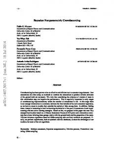
3.3. Simulated example We replicate the results reported by Dunson et al. (2007a), where a different approach is proposed. Following Dunson et al. (2007a), we simulate n = 500 observations from a mixture of two normal linear regression models, with the mixture weights depending on the predictor, different error variances and a non-linear mean function for the second component, ind.

yi | xi ∼ exp{−2xi }N (yi |xi , 0.01) + (1 − exp{−2xi }) N (yi |x4i , 0.04), i = 1, . . . , n. iid

The predictor values xi are simulated from a uniform distribution, xi ∼ U (0, 1). The following code is useful to plot the true conditional densities and the mean function: R> dtrue mtrue R> R> R> R> R> R> R>

set.seed(0) nrec R> R> R> +

library("splines") W R> +

par(cex = 1.5, mar = c(4.1, 4.1, 1, 1)) plot(fitLDDP$grid, fitLDDP$densp.h[6,], lwd = 3, type = "l", lty = 2, main = "", xlab = "y", ylab = "f(y|x)", ylim = c(0, 4)) lines(fitLDDP$grid, fitLDDP$densp.l[6,], lwd = 3, type = "l", lty = 2) lines(fitLDDP$grid, fitLDDP$densp.m[6,], lwd = 3, type = "l", lty = 1) lines(fitLDDP$grid, dtrue(fitLDDP$grid, xpred[6]), lwd = 3, type = "l", lty = 1, col = "red")

Finally, both functions return the posterior mean estimates and the limits of point-wise 95% HPD intervals for the mean function in the model objects meanfp.m, and meanfp.l and meanfp.h, respectively. The following code was used to obtain the estimated mean function under the LDDP model, along with the true function. R> R> R> R> R> R>

par(cex = 1.5, mar = c(4.1, 4.1, 1, 1)) plot(x, y, xlab = "x", ylab = "y", main = "") lines(xpred, fitLDDP$meanfp.m, type = "l", lwd = 3, lty = 1) lines(xpred, fitLDDP$meanfp.l, type = "l", lwd = 3, lty = 2) lines(xpred, fitLDDP$meanfp.h, type = "l", lwd = 3, lty = 2) lines(xpred, mtrue(xpred), col = "red", lwd = 3)

4. Mixed-effects models with nonparametric random effects Standard implementations of generalized linear mixed models (GLMM) typically assume independent and identically distributed random effects from a parametric distribution. Different BNP strategies have been proposed to relax the parametric assumption, including DP, DPM of normals, and PT (see, Jara, Hanson, and Lesaffre 2009, for a review and methods based on PT), which are available in the current version of DPpackage. In this section we show how to fit a semiparametric GLMM using the PTglmm function. The example further illustrates that a proportional-hazards model with nonparametric frailties can be fitted using any of the BNP-GLMM functions.

4.1. A semiparametric GLMM Assume that for each of m experimental units the regression data (Yij , xij , z ij ), 1 ≤ i ≤ m, 1 ≤ j ≤ ni , is recorded, where Yij is a response variable, and xij ∈ Rp and z ij ∈ Rq are p- and q-dimensional design vectors, respectively. The observations are assumed to be conditionally independent with exponential family distribution, p (Yij | ϑij , τ ) = exp {[Yij ϑij − b(ϑij )] /τ } c (Yij , τ ) .

Journal of Statistical Software

13

2 = V ar (Y | ϑ , τ ) are related to the The means µij = E (Yij | ϑij , τ ) and variances σij ij ij 0 2 = τ b00 (ϑ ), respectively. canonical ϑij and dispersion parameter τ via µij = b (ϑij ) and σij ij The means µij are related to the p-dimensional and q-dimensional “fixed” effects vectors β F and β R , respectively, and the q-dimensional “random” effects vector bi via the link relation F > R > h(µij ) = ηij = x> ij β + z ij β + z ij bi ,

(3)

where, h(·) is a known monotonic differentiable link function, and ηij is called the linear predictor. Due to software limitations, the analyses are often restricted to the setting in which the iid random effects follow a multivariate normal distribution, b1 , . . . , bm | Σ ∼ Nq (0, Σ). BNP extensions incorporate a probability model for the random effects distribution in order to better represent the distributional uncertainty and to avoid the effects of the miss-specification of an arbitrary parametric random effects distribution. Under these approaches, the parametric assumption is relaxed by considering iid

b1 , . . . , bm | G ∼ G, and G | H ∼ H, where H is one of the previously mentioned probability models for probability distributions (e.g., DP, DPM, PT). Even though any of the BNP models can be considered with this aim, its implementation is not direct and it is necessary to discuss some important issues regarding the specification of the model. Specifically, it is important to stress that under parameterization given by expression (3), β R represents the mean of random effects, and bi represents the subject-specific deviation from the mean. It follows that fixing the mean of the normal prior distribution for the random effects b at zero in the parametric context corresponds to an identification restriction for the model parameters (see, e.g., Newton 1994; San Mart´ın, Jara, Rolin, and Mouchart 2011). Equivalently, the random probability measure must be appropriately restricted in a semiparametric GLMM specification. In our settings, the location of G is “confounded” with the parameters β R . Although such identification issues present no difficulties for a Bayesian analysis in the sense that a prior is transformed into a posterior using the sampling model and the probability calculus, if the interest focuses on a “confounded” parameter, then such formal assurances have little practical value. Furthermore, as more data become available, the posterior mass will not concentrate on a point in the model, making asymptotic analysis difficult. As pointed out by Newton (1994), from a computational point of view, identification problems imply ridges in the posterior distribution and MCMC methods can be difficult to implement in these situations. Following Jara et al. (2009), we consider the following re-parameterization of the model > ηij = x> ij β + z ij θ i ,

iid

θ 1 , . . . , θ m | G ∼ G, and G|H∼H

14

DPpackage: Bayesian Semi- and Nonparametric Modeling in R

where β = β F , and θ i = β R +bi , and we center the nonparametric priors for G at an Nq (µ, Σ) distribution. Notice that samples under the original parameterization can be obtained in a straightforward manner from the MCMC samples, as discussed by Jara et al. (2009). When a DP or DPM prior is used to model the random effects distribution, Dunson, Yang, and Baird (2007b) and Li, M¨ uller, and Lin (2007) proposed alternative strategies to avoid the identifiability problem described above, but these approaches are not implemented in the current version of DPpackage. The PTglmm function considers the PT prior for G as described in Jara et al. (2009), such that G | α, µ, Σ, O ∼ P T M (Πµ,Σ,O , Aα ), where M is the maximum level of the partition to be updated, Πµ,Σ,O = {πj }j≥0 is a set of partitions of Rq , indexed by the centering mean µ, centering covariance matrix Σ and the matrix O, and Aα is a family of non-negative vectors controlling the variability of the process indexed by α > 0. Here O is a q × q orthogonal matrix defining the “direction” of the partition sets and the PT prior is centered around Nq (µ, Σ) distribution. The models in PTglmm are completed by assuming the following prior distributions:
β ∼ Np β 0 , S β0 , τ −1 |τ1 , τ2 ∼ Γ (τ1 /2, τ2 /2) , µ | µb , S b ∼ Nq (µb , S b ) , Σ | ν0 , T ∼ IWk (ν0 , T ) , O ∼ Haar(q), and α | a0 , b0 ∼ Γ (a0 , b0 ) , where Γ, IW , and Haar refer to the Gamma, inverted Wishart, and Haar distributions, respectively. Notice that the inverted Wishart prior is parameterized such that E(Σ) = T −1 /(ν0 − q − 1). Notice also that the Haar measure induces a uniform prior on the space of the orthogonal matrices.

4.2. A proportional hazards model with nonparametric frailties We show that DPpackage functions for fitting GLMM can be used to fit the Cox proportional hazards model (Cox 1972) with nonparametric frailties in this section. Consider right-censored survival data where failure times are repeatedly observed within a group or subject. Let i = 1, . . . , n denote the strata over which repeated times-to-event are recorded, and j = 1, . . . , ni denote the repeated observations within stratum i. The data are denoted by {(wij , tij , δij ) : i = 1, . . . , n, j = 1, . . . , ni }, where tij is the recorded event time, δi = 1 if tij is an observed

Journal of Statistical Software

15

failure time and δij = 0 if the failure time is right censored at tij , and wij is a p-dimensional vector of covariates. The baseline hazard function λ0 (t) corresponds to an individual with covariates w = 0 and survival time T0 . Given that the baseline individual has made it up to t, T0 ≥ t, the baseline hazard is how the probability of expiring in the next instant is changing. In terms of the baseline survival function S0 (t) = P (T0 > t) and density f0 (t), this is given by P (t ≤ T0 < t + |T0 ≥ t) f0 (t) = .  S0 (t)

λ0 (t) = lim

→0+

The conditional proportional hazards assumption stipulates that λ(tij |z ij ) = λ0 (t) exp(w> ij γ + θi ), where θ = (θ1 , . . . , θn )> are random effects, termed frailties in the survival literature. Often the frailties θi , or exponentiated frailties eθi , are assumed to be iid from some parametric distribution such as N (0, σ 2 ), gamma, positive stable, etc. We consider a PT prior for the frailties distribution below. The specification is conditional because proportionality only holds for survival times within a given group i, not across groups unless the distribution of θi is positive stable (see, e.g., Qiou, Ravishanker, and Dey 1999). Precisely, for individuals j1 and j2 within group i, λ(tij1 |wij1 ) = exp{(wij1 − wij2 )> γ}. λ(tij2 |wij2 ) Often the baseline hazard is assumed to be piecewise constant on a partition of R+ comprised of K intervals, yielding the piecewise exponential model. References are too numerous to list. See, for instance, Walker and Mallick (1997), Aslanidou, Dey, and Sinha (1998), and Qiou et al. (1999). Assume that λ0 (t) =

K X

λk I{ak−1 < t ≤ ak },

k=1

where a0 = 0 and aK = ∞, although in practice aK = max{tij } is sufficient. The prior > hazard is specified by cutpoints {ak }K k=0 and hazard values λ = (λ1 , . . . , λK ) . If the prior on λ is taken to be independent gamma distributions, the model can approximate the gamma process on a fine mesh (Kalbfleisch 1978). Regardless, the resulting model implies a Poisson likelihood for “data” yijk , taking values yijk = 0 when tij ∈ / (ak−1 , ak ] or δij = 0, and yijk = 1 when tij ∈ (ak−1 , ak ] and δij = 1, for k = 1, . . . , K(tij ), where K(t) = max{k : ak ≤ t}. The likelihood for (β, λ, γ) is given by

L(β, λ, γ) =

ni n Y Y

K(tij )

Y 

i=1 j=1

∝



 h iδij > log{λK(tij ) }+w> ij β+γi e− exp{log(λk )+wij β+γi }∆ijk  e ,

k=1

ni K(t n Y Y Yij ) i=1 j=1 k=1

p(yijk |µijk ),

16

DPpackage: Bayesian Semi- and Nonparametric Modeling in R

where p(y|µ) is the probability mass function for a Poisson(µ) random variable, µijk = exp{log(λk ) + w> ij β + γi }∆ijk , and ∆ijk = min{ak , tij } − ak−1 . Thus, the Cox model assuming a piecewise constant baseline hazard can be fitted in any software which allows for Poisson regression. Note that if covariates are time dependent as well, and change only at values included in {ak }K k=0 , the likelihood is trivially extended to include w ijk above for k = 1, . . . , K(tij ), rather than wij .

4.3. Kidney patient data We consider data on n = 38 kidney patients discussed by McGilchrist and Aisbett (1991). Each of the patients provides ni = 2 infection times, some of which are right censored. McGilchrist and Aisbett (1991) found that only gender was significant, and so we follow Aslanidou et al. (1998), Walker and Mallick (1997), Qiou et al. (1999), and Hemming and Shaw (2005) in considering only this covariate in what follows. We fitted the semiparametric proportional hazards regression model using a nonparametric prior for the frailties distribution. The commands used to prepare the data to fit the model are given in the supplementary material. The original dataset, d[i, j], is a 38 by 6 matrix, which for each row (from left to right) contains the subject indicator, ti1 , δi1 , ti2 , δi2 , and the gender indicator. Ten intervals were considered with cutpoints {a1 , . . . , a10 } taken from the empirical distribution of the data. We performed the analysis using the PTglmm function for the responses y i = (yi11 , . . . , yi1K(ti1 ) , . . . , yi21 , . . . , yi2K(ti2 ) ), where xij is a 11-dimensional design vector containing the gender indicator and the indicator for the interval associated with the corresponding response. Finally, we set β > = (γ > , λ> ), and assume 2

G ∼ P T M (Πσ , Aα ). We consider a M = 5 finite PT prior which was centered around a N (0, σ 2 ) distribution and constrained to have median-0 (frstlprob = TRUE in the prior object below). The values for the hyper-parameters β 0 and S β0 were obtained from a penalized quasi-likelihood (PQL) fit, using the glmmPQL function available from the MASS package (Venables and Ripley 2002). The matrix S β0 was inflated by a factor of 100. The remaining hyper-parameters were a0 = b0 = 1, ν0 = 3, and T = I 1 . The following code illustrate the prior specification: R> R> + R> R> R> +

library("MASS") fit0

fitPT