Drawing huge graphs by algebraic multigrid optimization

DRAWING HUGE GRAPHS BY ALGEBRAIC MULTIGRID OPTIMIZATION YEHUDA KOREN∗ , LIRAN CARMEL∗ , AND DAVID HAREL∗ Abstract. We present an extremely fast graph drawing algorithm for very large graphs, which we term ACE (for Algebraic multigrid Computation of Eigenvectors). ACE exhibits a vast improvement over the fastest algorithms we are currently aware of; using a serial PC, it draws graphs of millions of nodes in less than a minute. ACE finds an optimal drawing by minimizing a quadratic energy function. The minimization problem is expressed as a generalized eigenvalue problem, which is solved rapidly using a novel algebraic multigrid technique. The same generalized eigenvalue problem seems to come up also in other fields, hence ACE appears to be applicable outside graph drawing too. Key words. algebraic multigrid, multiscale/multilevel optimization, graph drawing, generalized eigenvalue problem, Fiedler vector, force directed layout, the Hall energy

1. Introduction. A graph is a structure G(V, E) representing a binary relation E over a set of entities V. In a very general sense, we expect the drawing of a graph to visually capture its inherent structure. Interpreting this vague desire as strict welldefined criteria for the purpose of assessing the quality of a drawing can be done in various ways, leading to many approaches to graph drawing [6, 18]. One of the most popular approaches is to define an energy function (or a force model), whose minimization determines the optimal drawing. Several such functions have been proposed, e.g., in [7, 16, 5, 8], each characterized by a different set of properties. In this paper we concentrate on one particular form of the energy function, characterized by being simple and smooth, thus enabling rigorous analytical analysis and a straightforward implementation. This particular function was first applied to graph drawing by Hall [11], and we therefore term it Hall’s energy. Most graph drawing methods suffer from lengthy computation times when applied to really large graphs. Several publications in the graph drawing conference of 2000 [12, 26, 9, 22] present fast graph drawing algorithms, but even the fastest of them ([26]) requires about 10 minutes for a typical 105 -node graph. As far as we know, no faster algorithm has been presented since. In fact, a naive implementation of the minimization of Hall’s energy would also encounter real difficulties on a 10 5 node graph. In this paper we suggest an extremely fast algebraic multigrid (AMG) [3, 4, 23, 25] implementation for minimizing Hall’s energy. It results in typical computation times of 10-20 seconds for 106 -node graphs. Actually, we suggest not only an implementation, but rather a generalization of the original method, allowing for the drawing of a much larger family of graphs (graphs with masses and negative weights, to be precisely defined later). Furthermore, the problem that we will be solving is of more fundamental nature, and our algorithm can be used in areas outside of graph drawing, such as clustering, partitioning, ordering, and image segmentation. In Section 2 we describe the original method proposed by Hall. In Section 3 we develop ACE, and investigate its features. Section 4 presents the results of many tests that we have been running, demonstrating the capabilities of the algorithm. A discussion follows in Section 5. Appendix A addresses related issues of graphconnectivity. ∗ The Weizmann Institute of Science, Rehovot 76100, {yehuda,liran,dharel}@wisdom.weizmann.ac.il Fax. +972-8-9342945

1

Israel.

E-mail:

2

Y. Koren, L. Carmel and D. Harel

2. The Eigenprojection Method. In this section we briefly introduce the original method of energy minimization proposed by Hall [11] using a somewhat different derivation. For a more detailed presentation the reader is referred to [19]. We will call this method as the eigenprojection method, for reasons that will become clear shortly. A graph is usually written G(V, E), with V = {1, . . . , n} a set of n nodes, and E a set of weighted edges. The weight of the edge connecting nodes i and j reflects their similarity, and is denoted by wij ≥ 0. Henceforth, we shall assume wij = 0 for any non-adjacent pair of nodes, and that there are no self-edges (i.e., wii = 0 for all i). def P The degree of node i is defined as di = j wij . The Laplacian, L, is a symmetric positive semi-definite n × n matrix associated with a graph, which is of fundamental importance to this work. It is defined as  di i=j i, j = 1, . . . , n. Lij = −wij i 6= j For a connected graph L has one and only one zero eigenvalue, which is associated def with the eigenvector 1n = (1, 1, . . . , 1)T ∈ Rn . Throughout the paper we assume, without loss of generality, that G is connected (if it is not, each connected component can be drawn separately). The usefulness of the Laplacian stems from the fact that the quadratic form associated with it is just a weighted sum of all the pairwise squared distances: Lemma 2.1. Let L be an n × n Laplacian, and let x ∈ Rn . Then 1X xT Lx = wij (xi − xj )2 . 2 i,j This lemma can be proved by direct expansion of the sum. Hall suggested to draw a graph G in one-dimension by minimizing this exact def quadratic form, E = xT Lx, to be denoted henceforth the Hall energy. Here, xk is the one-dimensional coordinate associated with the k’th node. Clearly, E ≥ 0 for any drawing and any graph. Intuitively, the larger the weight of the edge connecting nodes i and j, the closer xi and xj should be, in order to keep the contribution to the energy small. Given this function, the energy minimization strategy suggests that the coordinates be determined from: min xT Lx. x

(2.1)

However, this formulation of the graph drawing problem is not enough. The reason is that E is minimized (and takes the value 0) by solutions of the form x = c · 1 n with c being any constant. These solutions are undesirable from the graph drawing point of view, since they place all the nodes at the same location. These undesirable solutions can be avoided by requiring the drawing to have a finite variance, Var(x) = 1, meaning that the nodes are well-scattered. This is equivalent to replacing (2.1) with min xT Lx x

(2.2)

given xT x = 1 in the subspace xT · 1n = 0. The choice of a unit variance in the constraint is arbitrary. We could equally well choose a constraint of the form Var(x) = c, with c being any positive scalar. The

Drawing Huge Graphs by AMG Optimization

3

choice of c merely determines the length of x and√ the scale of E. For, if x0 is a minimizer of (2.2) with energy E0 = xT0 Lx0 , then cx0 (with energy cE0 ) will be a minimizer of the same problem but with the constraint Var(x) = c. Throughout the paper we use the convention 0 = λ1 < λ2 ≤ . . . ≤ λn for the eigenvalues of L (which are known to√be real), and denote the corresponding real orthonormal eigenvectors by v1 = (1/ n) · 1n , v2 , . . . , vn . It can be shown that the minimum of (2.2) is obtained for x = v2 , and the value of E at the minimum is λ2 . As a matter of fact, v2 is a vector of fundamental importance to many fields besides graph drawing; see, e.g., [21]. In fact, it has its own name — the Fiedler vector. Appropriately, we term (2.2) the eigenprojection problem. If it is desired to plot the graph in more dimensions, subsequent eigenvectors may be taken. Thus, a 2-D drawing is obtained by taking the x-coordinates of the nodes to be given by v 2 , and the y-coordinates to be given by v3 . Calculating the first few eigenvectors of L is a difficult task that presents a real problem for standard algorithms when n becomes around 105 . 3. The ACE Algorithm. In this section we describe our algorithm, ACE (Algebraic multigrid Computation of Eigenvectors), for solving the eigenprojection problem (2.2). In fact, as we shall see, ACE has a broader spectrum of applicability, being capable of solving a more general problem, the generalized eigenprojection problem. ACE employs a technique common to the so-called algebraic multigrid (AMG) algorithms [3, 4, 23, 25]. These algorithms progressively express an originally highdimensional problem in lower and lower dimensions, using a process called coarsening. On the coarsest scale the problem is solved exactly, and then starts a refinement process, during which the solution is progressively projected back into higher and higher dimensions, updated appropriately at each scale, until the original problem is reproduced. An AMG algorithm should be specifically designed for a given problem, so that the coarsening process keeps the essence of the problem unchanged, while the refinement process needs only fast updates to obtain an accurate solution at each scale. As far as we know, this is the first time that a formal and rigorous AMG algorithm is developed for graph drawing. Several authors, including some of us, have designed “heuristic” multiscale/multilevel graph drawing algorithms, i.e., algorithms in which the relationship between the problems on the different scales is not rigorously defined; see [10, 12, 26, 9]. Another important heuristic multiscale algorithm, from which we draw some of our inspiration, was developed by Barnard and Simon [1]. It computes the Fiedler vector for use in the partitioning problem. In Subsection 3.1 we derive the generalized eigenprojection problem. Our coarsening and refinement techniques are described in Subsections 3.2 and 3.3, respectively. Subsection 3.4 is devoted to the interpolation matrix — a key concept introduced later on. A schematic summary of the algorithm is given in Subsection 3.5. 3.1. The Generalized Eigenprojection Problem. In contrast to what AMG algorithms strive for, it will become apparent in Subsection 3.2 that the eigenprojection problem (2.2) is not preserved during coarsening. Hence, what we do is to define a different problem — the generalized eigenprojection problem — which is preserved during coarsening, and which contains the eigenprojection problem as a special case. ACE is designed to solve generalized eigenprojection problems, and thus also eigenprojection problems. Hence, we dedicate this first part to describe this generalized eigenprojection problem. One possible course of action would be to formulate it in a purely formal

4

Y. Koren, L. Carmel and D. Harel

fashion, expressing it as a problem in linear algebra. However, we take a different approach, and show how the generalized problem is tightly connected to graph theory and emerges naturally from trying to draw a more general entity, that we shall be calling a PSD graph. Definition 3.1 (Positive Semi-Definite (PSD) Graph). A PSD graph is a structure G(V, E, M) in which: 1. V = {1, . . . , n} is a set of n nodes. 2. E is a set of weighted edges, wij being the weight of the edge connecting nodes i and j. The weights wij satisfy the following rules: • The Laplacian of G is positive semi-definite. • wii = 0 ∀i (no self-edges). • wij = 0 for i, j non-adjacent pair. 3. M is a set of n strictly positive masses, mi being the mass of the i’th node. A PSD graph differs from a classical graph in two aspects. First, it involves an additional set of numbers — the masses. Second, we have fewer restrictions on the weights — instead of requiring them to be all positive (see section 2), we allow negative weights, as long as the Laplacian remains positive semi-definite. For the purpose of graph drawing, positive weights are interpreted as measuring the similarity between pairs of nodes — the larger wij the more similar are nodes i and j. In analogy we might interpret negative weights as measuring dissimilarity — the larger −w ij the more dissimilar are nodes i and j. Consequently, in the drawing we would expect nodes connected by large positive weights to be close to each other, and those connected by large negative weights to be distantly located. A zero weight wij thus expresses indifference as to the relative locations of nodes i and j. With this interpretation in mind, minimization of Hall’s energy, E = xT Lx, still looks like a good drawing strategy. But why do we need to assure positive semi-definiteness of the Laplacian? Because otherwise we can find x such that the energy is negative; xT Lx < 0. But then, stretching the coordinates by a constant factor, say by c > 0, will further decrease the energy, c2 xT Lx < xT Lx < 0. Consequently, as x is stretched towards infinity, the energy will decrease to minus infinity. Physically, such graphs are not interesting, and we do not expect to find them in real problems. We may safely rule them out. We are aware of the fact that negative weights might seem unnatural, but we hope that our work might demonstrate that graphs with negative weights can be as natural and legitimate as conventional ones. Since we are going to frequently address the issue of negative versus positive weights, we find it convenient to use a special name for the case of a PSD graph with no negative weights: Definition 3.2 (All-Positive (AP) Graph). A PSD graph G(V, E, M) is called all-positive if all its weights are non-negative. Due to the positive semi-definiteness of the Laplacian, negative weights will always be inferior to positive ones. This is an important observation that we now prove: Claim 3.1. Let G(V, E, M) be a PSD graph. The degree of each of its nodes is non-negative. Proof. The diagonal elements of the Laplacian are the degrees, so our claim is just a re-statement of a well known property of positive semi-definite matrices, saying that all the diagonal elements are non-negative. To prove this let us assume that one node, say the first, has d1 < 0. Then, if we take x = (1, 0, 0, . . . , 0)T , P P a negative degree, 1 2 we get E = 2 i,j wij (xi − xj ) = j w1j = d1 < 0, and so L cannot be positive semi-definite. So far, we saw that the function to be minimized, Hall’s energy, did not change if

Drawing Huge Graphs by AMG Optimization

5

we deal with PSD graphs. The deviation from Hall’s formulation is in the constraints. To this end we define the mass matrix as follows: Definition 3.3 (Mass Matrix). Let G(V, E, M) be an n-node PSD graph. The n × n diagonal matrix M , defined by  0 i 6= j Mij = mi i = j, is called the mass matrix of G. Using this matrix, we replace problem (2.2) by weighting sums according to node masses, to obtain: min xT Lx x

(3.1)

given xT M x = 1 in the subspace xT M · 1n = 0. In the next section we will see that this form of the constraints is a natural outcome of the coarsening process, and for all practical reasons it suffices to take it as such. Moreover, weighting by masses is proved more natural in various problems. For example, in many cases minimizing (3.1), where the masses are taken as the node degrees, is the preferred strategy, e.g., [24, 19]. Throughout the paper we use the convention 0 = µ1 < µ2 ≤ . . . ≤ µn for the generalized eigenvalues of (L, M ) (which are known to be real), and denote the corresponding real orthonormal eigenvectors by u1 = α · 1n , u2 , . . . , un (α some constant). It can be shown that the minimum of (3.1) is obtained for x = u2 , and the value of E at the minimum is µ2 . Appropriately, we term (3.1) the generalized eigenprojection problem. If it is desired to plot the graph in more dimensions, subsequent eigenvectors may be taken. Thus, a 2-D drawing is obtained by taking the x-coordinates of the nodes to be given by u2 , and the y-coordinates to be given by u3 . Since it is obvious from Definition 3.1 that both the Laplacian L and the mass matrix M completely define a PSD graph,1 we will freely use both G(V, E, M) and G(L, M ) to denote a PSD graph. Clearly, the eigenprojection problem is just a special case of the generalized eigenprojection problem, given that the graph is an AP graph, and given that all the masses are 1. 3.2. The Coarsening Process. During the coarsening, we iteratively represent an initial PSD graph as a sequence smaller and smaller PSD graphs. Let G be such a PSD graph containing n nodes. A single coarsening step would be to replace G with another PSD graph Gc , containing only m < n nodes (typically, m ≈ 21 n). Of course, the structure of Gc should be strongly linked to that of G, such that both describe approximately the same entity, but on different scales. One can think of many clever ways to erect Gc given the structure of G, but we postpone discussion on this topic until Subsection 3.4. Instead, we establish a general framework for the coarsening, into which later specific methods can be easily cast. A key concept we will use is that of an interpolation matrix, which is the tool that links G and Gc . This is an n × m matrix P that interpolates m-dimensional vectors y ∈ Rm into n-dimensional ones x = P y (x ∈ Rn ). If y is the solution of the generalized eigenprojection problem of Gc , a good interpolation matrix is one 1 Actually,

this is true as long as we are given a definite order 1, . . . , n of the nodes.

6

Y. Koren, L. Carmel and D. Harel

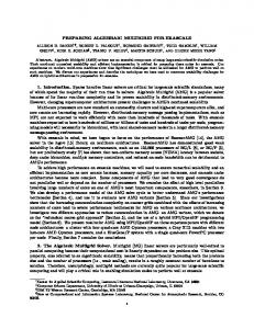
for which x = P y is close enough to the solution of the generalized eigenprojection problem of G. Such interpolation matrices can be designed in various ways, to be discussed, as already mentioned, in Subsection 3.4. In the meantime we just state the general definition of P : Definition 3.4 (Interpolation Matrix). An interpolation matrix P is an n × m matrix (n > m) such that 1. All elements are non-negative:PPij ≥ 0 ∀i, j. m 2. The sum of each row is one: j=1 Pij = 1 ∀i. 3. P has a full column rank: rank(P ) = m. Properties 1 and 2 follow naturally by interpreting the i’th row of P as a series of weights that shows how to determine coordinate xi given all the y’s, namely, xi = Pm P y . Property 3 prevents the possibility of two distinct m-dimensional vectors ij j j=1 being interpolated to the same n-dimensional vector. Since 1n = P ·1m (from property 2), we are thus assured that no “good” drawing of Gc will be interpolated to the undesirable drawing of G, α · 1n . In Appendix A we show that the fact that P is of full column rank also has a role in issues of graph connectivity. The interpolation matrix defines a coarsening step completely: Given a fine nnode PSD graph G(L, M ) and an n × m interpolation matrix P , we can fully obtain the coarse m-node PSD graph Gc (Lc , M c ). Put differently, given L, M and P , we calculate the Laplacian Lc , and the mass matrix M c . In the rest of this subsection we show how we do it: In 3.2.1 we explain how M c is found, and in 3.2.2 we explain how Lc is found. Finally, in 3.2.3 we discuss the relations between the generalized eigenprojection problem of Gc and that of G. Before we start, however, let us introduce a simple example upon which we demonstrate the subsequent results. Let the fine graph G be the 5-node PSD graph (actually, AP graph) shown in Figure 3.1. Due to its structure, this graph will be henceforth dubbed the Eiffel tower graph. Let all the masses of G be 1, so that its Laplacian and mass matrix are given by:     9 −5 0 −4 0 1 0 0 0 0  −5 17 −2 −7 −3   0 1 0 0 0         L =  0 −2 4 −2 0  M =  (3.2)  0 0 1 0 0 .  −4 −7 −2 19 −6   0 0 0 1 0  0 −3 0 −6 9 0 0 0 0 1 Let the interpolation matrix be the 5 × 3  0.55  0.52  P =  0.3  0.45 0.4

matrix 0 0 0.4 0 0

0.45 0.48 0.3 0.55 0.6



  .  

(3.3)

We would like to remind the reader that for the time being we assume that P is given in advance. Ways to build P given G(L, M ) are discussed only in Subsection 3.4. In any case, we can easily become convinced that this P is reasonable, since it fixes the first and third nodes of the resulting 3-node PSD graph Gc (10 and 30 ) as the coarse version of the “tower base” quadruplet (1,2,4,5), and the second node 2 0 as the coarse version of the “tower top”. 3.2.1. Calculating the mass matrix of Gc . The coarse masses are derived by:

Drawing Huge Graphs by AMG Optimization

7

3

2

2

7

2

4

5

6 4

3

5

1

Fig. 3.1. The Eiffel tower graph.

Definition 3.5 (Mass law). Let G be a fine n-node PSD graph with masses m1 , m2 , . . . , mn , and let P be an n × m interpolation matrix. The masses of the coarse PSD graph Gc mc1 , mc2 , . . . , mcm are given by mcj =

n X

Pij mi .

i=1

In 3.2.3 we will understand why this is a natural definition. In the meantime, let us just say that this law is nothing but a statement of mass conservation if we interpret the nodes of G as physical masses formed by breaking and re-fusing (as dictated by the interpolation matrix) pieces of the physical masses from which G c is built up. Applying the mass law to the Eiffel tower example, we get:   2.22 0 0 0.4 0 . Mc =  0 (3.4) 0 0 2.38

Notice that the total mass is indeed conserved, TrM = TrM c = 5. Next, we prove two useful equalities (which are basically just two variations on the same equality) that stem from the mass law, and will serve us later: Lemma 3.6. Let P be an n × m interpolation matrix, M be the n × n mass matrix of G, and M c be the corresponding m × m mass matrix of Gc . Then M c · 1m = P T M · 1n .

Proof. M · 1n is just (m1 , m2 , . . . , mn )T , and M c · 1m is just (mc1 , mc2 , . . . , mcm )T . Thus, (M c · 1m ) = P T (M · 1n ) is merely a matrix form of the mass law. Lemma 3.7. Let P be an n × m interpolation matrix, M be the n × n mass matrix of G, and M c the corresponding m × m mass matrix of Gc . Then, the sum of the i’th row (or column) of P T M P is just mci , or M c · 1m = P T M P · 1 m .

8

Y. Koren, L. Carmel and D. Harel

Proof. The rows of P all sum up to one, thus P · 1m = 1n . Replacing 1n by P · 1m in Lemma 3.6 completes the proof. 3.2.2. Calculating the Laplacian of Gc . The Hall energy of G(L, M ) is E = xT Lx, where x ∈ Rn . Substituting x = P y, we can express this energy in terms of the m-dimensional vector y, E = y T P T LP y. It would then be quite natural to define the Laplacian of Gc to be Lc = P T LP,

(3.5)

so that the Hall energy of Gc (Lc , M c ) is E = y T Lc y. The next claim shows that this definition is consistent with our previous definitions. Claim 3.2. Lc is the Laplacian of a PSD graph. Proof. We have to show that Lc is symmetric positive semi-definite, and that the sum of each of its rows is 0. The symmetry and positive semi-definiteness are imposed only by the fact that L is such: a. Symmetry: Notice that (Lc )T = (P T LP )T = P T LT P = P T LP = Lc . b. Positive semi-definiteness: Given any vector y ∈ Rm , let us denote by z ∈ Rn the vector P y. Then, y T Lc y = y T P T LP y = z T Lz, which is always non-negative due to the positive semi-definiteness of L. c Proving that the rows of Lc sum P up to 0 (L · 1m = 0) requires the use of the special features of P . The statement j Pij = 1 is equivalent to writing P · 1m = 1n . Then, Lc · 1m = P T LP · 1m = P T L · 1n = 0, where the last step is due to the fact that L · 1n = 0. Having found both Lc and M c , Gc is completely defined and the coarsening step comes to its end. Our definition of coarsening clarifies why we needed the concept of PSD graphs; negative weights might occur in Gc even if G is an AP graph. This actually happens in our Eiffel tower example, since we get   0.2788 −0.296 0.0172 0.64 −0.344  . Lc = P T LP =  −0.296 0.0172 −0.344 0.3268 This Laplacian, together with the mass matrix (3.4), defines the 3-node PSD graph Gc shown in Figure 3.2, with a negative weight connecting nodes 10 and 30 . The reason for the emergence of negative weights is delicate. Our definition of the coarse Laplacian, Lc = P T LP , has a tendency to diminish the value of a weight that connects two highly correlated coarse nodes, i.e., two coarse nodes that during the interpolation often contribute simultaneously to the same fine nodes. To see this, let us P examine explicitly the expression for the coarse weights. From (3.5) we obtain Lcij = p,q Ppi Pqj Lpq . Considering the definition of L, and separating the cases q = p and q 6= p, we get X X X Lcij = − Ppi Pqj wpq + Ppi Ppj wpq . p,q

p

q

The coarse weights are obtained from the off-diagonal elements of Lc . Using the notion of degree we get X X c = −Lcij = Ppi Pqj wpq − wij dp Ppi Ppj , i 6= j. (3.6) p,q

p

Drawing Huge Graphs by AMG Optimization

9

m2 = 0.4 2’

0.296

1’ m1 = 2.22

0.344

-0.0172

3’ m3 = 2.38

Fig. 3.2. The coarse version of the Eiffel tower graph.

The first term collects the contributions of all pairs hp, qi of fine nodes such that one is interpolated from i and the other from j. For an AP graph this term is always positive. The second term collects the contributions of those fine nodes for which both i and j contribute to their interpolation. But now, for any PSD graph this term c is always negative (see Claim 3.1), thus having the tendency to decrease w ij . In the 0 0 Eiffel tower example, nodes 1 and 3 are highly correlated, as can be seen by looking at the first and the third columns of P in (3.3), which explains the negative weight of the edge connecting them. 3.2.3. The eigenprojection solutions of G and Gc . Given the coarse graph G , its corresponding generalized eigenprojection problem is c

min y T Lc y y

(3.7)

given y T M c y = 1 in the subspace y T M c · 1m = 0, which we term the coarse generalized eigenprojection problem. The issue that needs to be addressed now is the relationship between this problem and the original generalized eigenprojection problem (3.1) of the fine graph G. To bring the two problems into the same dimension we substitute x = P y in (3.1), obtaining the form min y T P T LP y y

(3.8)

given y T P T M P y = 1 in the subspace y T P T M · 1n = 0, to be referred to as the restricted generalized eigenprojection problem. In general, the coarse generalized eigenprojection problem (3.7) and the restricted generalized eigenprojection problem (3.8) are different problems. Had these two problems been identical, then the multiscale method would be optimal in the sense that the structure of the problem is preserved during coarsening. As we will show in subsection 3.4, one can adopt strategies of choosing P such that this would indeed be the case. Yet other strategies, that may yield more powerful interpolation matrices, do not posses this property. Nevertheless, we will show that in these cases the coarse generalized eigenprojection problem (3.7) is a reasonable approximation of the restricted generalized

10

Y. Koren, L. Carmel and D. Harel

eigenprojection problem (3.8), and consequently the solutions of both problems share much resemblance. To start with, let us compare the two problems in more detail. Due to the equality Lc = P T LP , the function to be minimized is the same in both forms. Moreover, since M c · 1m = P T M · 1n (see Lemma 3.6), we are looking for solutions to both of these in the same subspace (i.e., in both we avoid the same undesirable solution). The only difference between them is in the scaling constraint, since in general M c 6= P T M P . In fact, we can formulate a simple criterion to decide, given P , whether M c = P T M P or not: Claim 3.3. Let G(L, M ) be an n-node PSD graph, and let P be an n×m interpolation matrix. The coarse generalized eigenprojection problem (3.7) becomes identical to the restricted generalized eigenprojection problem (3.8) if P T M P is diagonal.2 Proof. The two problems are identical if M c = P T M P . By Lemma 3.7, the sum of the i’th row (or column) of P T M P is just mci , so obviously M c = P T M P if P T M P is diagonal. In the case that M c 6= P T M P we would rather solve the coarse generalized eigenprojection problem than the restricted generalized eigenprojection problem, i.e., we would prefer working with M c over working with P T M P . This is for efficiency reasons, since matrix manipulations are always faster for diagonal matrices. So we work only with M c , and we now justify this by showing that the coarse generalized eigenprojection problem (3.7) arises naturally as an approximation of the restricted generalized eigenprojection problem (3.8). Let us start with the restricted generalized eigenprojection problem. As explained, the off-diagonal elements of P T M P slow down the computation, and therefore we have an interest in approximating the problem so as to conceal them. These elements are responsible for the fact that “mixed terms”, i.e., terms that involve the multiplication yi · yj for i 6= j, appear in the constraint y T P T M P y = 1. Expanding this constraint explicitly yT P T M P y =

X

mp Ppi Ppj yi yj ,

(3.9)

i,j,p

we notice that for the mixed terms to be non-zero, Ppi and Ppj should be non-zero simultaneously, implying a correlation between yi and yj . For any reasonable interpolation matrix, this means that yi and yj are not too distantly located. A good approximation, therefore, would be to replace each member in the pair yi and yj in (3.9) with the average 12 (yi + yj ). Thus, we have yi yj ≈

1 1 1 1 (yi + yj )2 = yi2 + yj2 + yi yj , 4 4 4 2

or yi yj ≈

1 2 (y + yj2 ). 2 i

2 As a matter of fact, one can show that P T M P will be diagonal if and only if P has exactly one non-zero element in each row.

11

Drawing Huge Graphs by AMG Optimization

Substituting this in (3.9) gives 1X mp Ppi Ppj (yi2 + yj2 ) = 2 i,j,p

yT P T M P y ≈

1X 1X mp Ppi Ppj yi2 + mp Ppi Ppj yj2 . 2 i,j,p 2 i,j,p

=

The two last terms are actually the same, so that yT P T M P y ≈

X

mp Ppi Ppj yi2 =

i,j,p

X i,p



mp Ppi yi2 

X j



Ppj  =

X

mp Ppi yi2 ,

i,p

where the last step is due to the fact that the sum of each row of any interpolation matrix is 1. Using further the mass law, we get ! X X X T T 2 y P MPy ≈ yi mp Ppi = mci yi2 = y T M c y, p

i

i

which is just the result that we wanted to prove. 3.3. The Refinement Process. We now keep coarsening further and further until we obtain a coarse PSD graph that is sufficiently small. Typically, we would stop the process when we have less than 100 nodes (the speed of the ACE algorithm does not depend on the exact value of this threshold). The drawing of G(L, M ), the coarsest graph, is obtained from the lowest positive generalized eigenvectors of (L, M ), namely u2 , u3 , . . .. Actually, we can write the problem as an eigenvalue problem in the form Bv = µv, 1

1

1

(3.10)

where B = M − 2 LM − 2 and v = M 2 u, which calls for finding the lowest positive eigenvectors of B. This is a classical problem that can be handled by numerous algorithms, such as QR and Lanczos (see, e.g., [27]). Due to the small size of B, finding its eigenvectors takes a negligible fraction of the total running time, which makes the choice of the algorithm a marginal issue. We chose to use a variation of the power iteration (PI) algorithm (see, e.g., [27]), which is designed for finding the largest eigenvectors (i.e., those associated with the eigenvalues of the largest magnitude) of symmetric matrices. For S a symmetric matrix, its largest eigenvector is the asymptotic direction of Sv0 , S 2 v0 , S 3 v0 . . ., where v0 is an initial guess. The next largest eigenvectors can be found using the same technique, taking v0 orthogonal to the previously found (larger) eigenvectors. Our problem needs the lowest eigenvectors rather than the largest ones. We therefore preprocess the matrix B, transforming it ˆ whose largest eigenvectors are identical to the lowest eigeninto a different matrix, B, vectors of B (see also [2]). This is done using the Gershgorin bound [27], which is a theoretical upper bound for (the absolute value of) the largest eigenvalue of a matrix. Specifically, for our matrix this bound is given by:   X g = max Bii + |Bij | . i

j6=i

12

Y. Koren, L. Carmel and D. Harel

ˆ = g · I − B has the same eigenvectors as B, but in reverse order — the The matrix B largest eigenvectors have become the lowest ones. Consequently, it is now suitable for using with the PI algorithm. The pseudocode of this algorithm is given in Figure 3.3. The initial guesses u ˆ2 , u ˆ3 , . . . are picked at random. PI seems to be a good algorithm to use here, being intuitive, simple to implement, having guaranteed convergence to the right eigenvector, and most of all suitable for the refinement process too. Given a certain eigenvector of B, say vi , we are able to calculate the generalized eigenvector 1 ui from ui = M − 2 vi . Function power iteration ({ˆ u2 , u ˆ3 , . . . , u ˆp }, L, M ) % {ˆ u2 , u ˆ3 , . . . , u ˆp } are initial guesses for {u2 , u3 , . . . , up }

% L, M are the Laplacian and mass matrix of the graph %  is the tolerance. We recommend using 10−7 ≤  ≤ 10−10 1

v1 ← M 2 · 1 n % first (known) eigenvector v1 ← kvv11 k % normalize the first eigenvector 1 1 B ← M − 2 LM − 2 g ← Gershgorin(B) ˆ ← g · I − B % reverse order of eigenvalues B for i = 2 to p 1 ˆi vˆi ← M 2 u v ˆi vˆi ← kˆvi k repeat vi ← vˆi % orthogonalize against previous eigenvectors

for j = 1 to i − 1 vi ← vi − (viT vj )vj end for ˆ · vi % power iteration vˆi ← B vˆi ← kˆvvˆii k % normalization until vˆi · vi > 1 −  % halt when direction change is negligible vi ← vˆi 1 u i ← M − 2 vi end for return u2 , . . . , up Fig. 3.3. The power iteration algorithm (PI).

Having solved the generalized eigenprojection problem for the coarsest PSD graph directly, we use the solution to accelerate the computation of the corresponding solution for the second coarsest PSD graph. We then proceed iteratively until the solution of the original problem is obtained. How is this ‘inductive step’, from the coarser to the finer graph, to be carried out? Well, let Gc (Lc , M c ) be a coarse m-node PSD graph, and let uc2 , uc3 , . . . ucp be the first few solutions of its generalized eigenprojection problem. For two-dimensional drawings uc2 and uc3 are all that we need (thus p = 3), but we do not specify p in order to keep the algorithm general. Let the next fine n-node PSD graph be G(L, M ), and let u2 , u3 , . . . , up be the first few solutions to its generalized eigenprojection problem. Let

Drawing Huge Graphs by AMG Optimization

13

also P be the n × m interpolation matrix connecting G and Gc . The refinement step uses uc2 , uc3 , . . . , ucp to obtain a good initial guess for u2 , u3 , . . . , up , thus enabling their fast calculation. The basic idea of the refinement is that for a reasonable interpolation matrix, u ˆi = P uci is a good approximation of ui . We then have to apply an iterative algorithm whose input is the initial guess u ˆi and whose output is the generalized eigenvector ui . The iterative algorithm that we use is the same power iteration that we have already used to solve the coarsest problem; see Figure 3.3. In an earlier version of ACE we used the Rayleigh quotient iteration (RQI) technique as an iterative algorithm for finding extreme eigenvectors. See details in the technical report version of this work [20]. A single iteration of RQI requires many computations (the solution of a system of linear equations), but on the other hand the convergence rate is extremely fast, and an accurate solution is obtained within a few iterations. In contrast, a single iteration of PI is very fast, but many more iterations are required. In general, the performance of both algorithms was quite similar, and we have chosen to use PI for two reasons: First, it is simple to implement and to track, and second, the convergence to the correct eigenvector is guaranteed (unlike RQI).

3.4. The Interpolation Matrix. At this point, the multiscale scheme is completely defined, and the only thing left unexplained is how we construct a specific interpolation matrix. More precisely, the question that we address here is: given an n-node PSD graph G(L, M ) that we would like to represent by a coarser, m-node, PSD graph Gc , what is an appropriate n × m interpolation matrix P ? As already mentioned, there is no unique recipe for this, and we can come up with many feasible methods. However, for the interpolation matrix to successfully fulfill its role, some guidelines should be followed: 1. The interpolation matrix should faithfully retain the structure of G, such that the initial guess P uci will be as close as possible to the desired solution ui . The way to achieve this is to construct P such that the Hall energy associated with P uci will be as low as possible. This is the very core of the multiscale scheme, and thus it is the most important property of the interpolation matrix. 2. The interpolation matrix should be fast to calculate, much faster than solving the generalized eigenprojection problem of the fine graph directly. Otherwise, we have done nothing in speeding up the calculation. 3. The sparser the interpolation matrix the better, since matrix manipulations will be faster. In a single coarsening step the coarse Laplacian Lc is determined from the fine one, L, by Lc = P T LP . Therefore, to preserve sparsity of the Laplacian we need a sparse interpolation matrix. Generally speaking, these guidelines are contradicting. Improving the preservation of the structure of a graph requires more accurate interpolation, and hence a denser and more complex matrix P . A good interpolation matrix thus reflects a reasonable compromise regarding the tradeoff between accuracy and simplicity. We now describe the two methods we have been using to construct P . To be able to compare these algorithms, we apply them to the Eiffel tower graph, and then compare the interpolated vectors P uci to the exact ones ui . The ui ’s were calculated by solving the generalized eigenprojection problem of the Eiffel tower graph directly.

14

Y. Koren, L. Carmel and D. Harel

Here are the first two: 

  u2 =   

0.2947 0.1354 −0.8835 0.1513 0.3021





  u3 =   

    

−0.6961 −0.0968 0.0080 0.0777 0.7071



  ,  

(3.11)

and they give rise to the drawing plotted in Figure 3.4. 0.8

5 0.6 0.4

u3

0.2

4

3 0

2

-0.2 -0.4 -0.6

1 -0.8 -1

-0.8

-0.6

-0.4

-0.2

0

0.2

0.4

u2 Fig. 3.4. The drawing of the Eiffel tower example obtained by direct solution of the generalized eigenprojection problem.

3.4.1. Edge contraction interpolation. In this method we interpolate each node of the finer graph from exactly one coarse node. To find an appropriate interpolation matrix, we first divide the nodes of the fine graph into small disjoint connected subsets, and then associate the members of each subset with a single coarse node. Consequently, the rows of all the members of the same subset in the interpolation matrix will be identical, having a single non-zero element (which is, of course, 1). In the Eiffel tower example, reasonable subsets would be {1, 2}, {3}, and {4, 5}, giving rise to the interpolation matrix

Pcon



  =  

1 1 0 0 0

0 0 1 0 0

0 0 0 1 1



  ,  

where the subscript con stands for contraction. A well known method to efficiently create such disjoint subsets is by contracting edges that participate in max-matching (see, e.g., [26, 17]), so that each two contracted nodes are interpolated from the same single coarse node. Here, in the Eiffel tower example, we have contracted the pairs {1, 2} and {4, 5}. Using the interpolation matrix Pcon , we obtain a coarse PSD graph Gc charac-

15

Drawing Huge Graphs by AMG Optimization

terized by the Laplacian and mass matrix   16 −2 −14 4 −2  Lccon =  −2 −14 −2 16

c Mcon



2 = 0 0

0 1 0

 0 0 . 2

c Solving the generalized eigenvalue problem for Lccon and Mcon directly, we get     −0.5 0.2236 uc3 =  0  . uc2 =  −0.8944  0.5 0.2236

Interpolating back yields the following approximations for the exact u 2 and u3 :     −0.5 0.2236  −0.5   0.2236      0 c 0 c    u3 = Pcon u3 =  u2 = Pcon u2 =  −0.8944   0 .  0.5   0.2236  0.5 0.2236

To evaluate how good these approximations are, we calculated the angles between them and the exact generalized eigenvectors (of which only u2 and u3 are given here explicitly; see (3.11)): ^(u02 , u1 ) = 90◦ ^(u02 , u2 ) = 8.9473◦ ^(u02 , u3 ) = 89.4852◦ ^(u02 , u4 ) = 81.1724◦ ^(u02 , u5 ) = 88.6478◦

^(u03 , u1 ) = 90◦ ^(u03 , u2 ) = 89.3327◦ ^(u03 , u3 ) = 37.9197◦ ^(u03 , u4 ) = 83.0270◦ ^(u03 , u5 ) = 52.9628◦

Clearly, u02 is close to u2 , and is almost orthogonal to all the others. Also, the closest vector to u03 is u3 , but in a less significant way; u03 almost lies on the plane defined by (u3 , u5 ), with a smaller angle with the u3 -axis than with the u5 -axis. The edge contraction method evidently prefers simplicity over accuracy. On the one hand, P is very sparse (each row contains exactly one non-zero element) and is easy to compute, but on the other hand, the interpolation is crude, taking into consideration only the strongest connection of each node. Indeed, we will see in Section 4 that this method is characterized by very fast coarsening, but yields less accurate interpolations during the refinement. The simple form of the resulting P gives rise to two elegant properties of the edge contraction algorithm, which we are about to prove: it preserves the structure of the problem, and it preserves the all-positiveness of the graph. Claim 3.4. Let G(L, M ) be an n-node PSD graph, and let P be an n×m interpolation matrix derived by the edge contraction algorithm. Then, the coarse generalized eigenprojection problem (3.7) is identical to the restricted generalized eigenprojection problem (3.8). Proof. By Claim 3.3 all we have to show is that P T M P is diagonal for any M . The ij’th element of P T M P is X (P T M P )ij = mp Ppi Ppj . p

16

Y. Koren, L. Carmel and D. Harel

But P has exactly one non-zero element in each row, so that Ppi Ppj is zero whenever i 6= j. Hence, (P T M P )ij = 0 for i 6= j. Indeed, it is easy to see that in the Eiffel tower example, M c = P T M P . Claim 3.5. Let G(L, M ) be an n-node AP graph, and let P be an n × m interpolation matrix derived by edge contraction. Then, the coarse graph G c will also be an AP graph. c Proof. Recall expression (3.6) for wij , the weights of Gc , c wij =

X p,q

Ppi Pqj wpq −

X

dp Ppi Ppj ,

p

i 6= j.

The second term vanishes, since in the previous proof we saw that Ppi Ppj = 0 for c i 6= j. Therefore, if ∀p, q wpq ≥ 0, then ∀i, j wij ≥ 0. Indeed, the coarse graph Gc of the Eiffel tower is an AP graph. 3.4.2. Weighted interpolation. In this method, inspired by common AMG techniques [3], we interpolate each node of the fine graph from possibly several coarse nodes. The first stage is to choose a subset of m nodes out of the n in G, such that they will be the nodes of Gc . Hereinafter, the elements of this subset will be called representatives. We pick the representatives using a technique that we have developed especially for this purpose. In order to properly explain this technique, we need further notations, to be defined next. Let R be the set of representatives, and let V −R be the set of non-representatives (recall that V denotes the set of all nodes). Since a representative i is uniquely associated with a coarse node, we denote this coarse node by [i]. For each nonrepresentative, we define the following two closely related magnitudes: Definition 3.8 (Partial Degree). The partial degree of a non-representative node i is X d0i = wik . k∈R

Definition 3.9 (Relative Connectivity). The relative connectivity of a nonrepresentative node i is ri =

d0i , di

where d0i is its partial degree and di its degree. The partial degree of a nonrepresentative is its degree with respect to the representatives only. The relative connectivity is an important notion that will also be used later on. For an AP graph 0 ≤ ri ≤ 1 ∀i, but for a general PSD graph, ri may take on any value. Equipped with these definitions, we can now describe the technique by which we pick the representatives; see Figure 3.5. The idea is to randomly order the nodes, and then to conduct a predetermined number of sweeps (typically two or three) along them, choosing as representatives those whose relative connectivity to the already chosen representatives is below a certain threshold. Naturally, the value of this threshold must be increased before a new sweep. Typically, we start with a threshold of 0.05, and then increase before each new sweep by 0.05. Having chosen the representatives, we are now ready to construct the interpolation matrix. We fix the coordinates of the representatives by their values as given in the

17

Drawing Huge Graphs by AMG Optimization

Function Find Representatives (V, t0 , tinc ) % V — the set of all nodes % t0 — the initial threshold value % tinc — the amount by which we increase the threshold in each new sweep

Build i1 , i2 , . . . , in , a random permutation of the nodes R←φ % Start with an empty set of representatives threshold ← t0 for i = 1, . . . , sweeps for p =P 1, . . . , n P rp ← k∈R wip k / k∈V wip k if rp < threshold R ← R∪{ip } end if end for threshold ← threshold + tinc end for return R Fig. 3.5. The technique to choose representatives for the weighted interpolation.

coarse problem. But then we adopt a different strategy to the interpolation of the non-representatives. Their coordinates are determined such that the total energy is minimized. To this end we write the Hall energy as: 1 X 1 X wij (xi − xj )2 = wij (xi − xj )2 + E= 2 2 i,j∈V

+

X X

i∈R j∈V−R

i,j∈R

wij (xi − xj )2 +

1 2

X

i,j∈V−R

wij (xi − xj )2 .

Let k ∈ V − R. Differentiating E with respect to xk gives X X ∂E wik (xi − xk ) wik (xi − xk ) − 2 = −2 ∂xk i∈R

i∈V−R

Equating this to zero and isolating xk , we get P P wik xi i∈R wik xi + Pi∈V−R xk = P i∈R wik + i∈V−R wik

k ∈ V − R.

k ∈ V − R.

(3.12)

(3.13)

This equation is satisfied by each of the non-representatives, and therefore (3.13) actually defines a set of n − m coupled equations. What we would really like to do, though, is to express the coordinates of each non-representative by those of the representatives. Indeed, it is possible in theory to work out this set of n−m equations such as to isolate the n−m coordinates of the non-representatives as functions of the m coordinates of the representatives. Yet in practice we should avoid it, for two reasons: First, it is overly time consuming. Second, it will result in a dense interpolation matrix, since each xk (k ∈ V − R) will depend on potentially many representatives. Therefore, to avoid lengthy computations and to save sparsity, we would like to approximate (3.13) by a simpler expression. Such an approximation might be achieved

18

Y. Koren, L. Carmel and D. Harel

if we ignore, when calculating xk , all other non-representatives, i.e., by taking them all as if they were located at xk . Due to the local nature of the interpolation, this is a reasonable approximation. For, if we look at the location of a particular nonrepresentative xk , then all the other non-representatives will be, on average, equally distributed around it. This assumption is equivalent to taking the second term in (3.12) to be zero. Taking a large enough relative connectivity threshold in the process of selecting representatives, we are assured that the term that we do not neglect (the first term in (3.12)) is indeed significant. Substituting xi = xk for i ∈ V − R in (3.13) gives P wik xi xk = Pi∈R k ∈ V − R. (3.14) i∈R wik Now, the elements of the interpolation matrix are just

wij Pi[j] = P i ∈ V − R, j ∈ R wik  k∈R 1 ifj = i i ∈ R. Pi[j] = 0 ifj 6= i

(3.15) (3.16)

This expression is much simpler and is fast to compute. It also results in a sparser interpolation matrix than we would have gotten from (3.13). If the result is still not sparse enough, we can always make it even sparser by interpolating xk only from the first few most dominant representatives. That is, for each k ∈ V − R we define a set R0k ⊆ R that includes at most r (a certain small number of) representatives, from which xk is interpolated. Equations (3.14) and (3.15) then become P i∈R0 wik xi xk = P k k ∈ V − R, (3.17) i∈R0 wik k

and

Pi[j] = P

wij k∈R0i

wik

i ∈ V − R, j ∈ R0i , R0i ⊆ R.

(3.18)

Obviously, if ∀k R0k = R, then (3.14) and (3.15) are reconstructed. Now we have guaranteed both sparsity and speed of computation, but we are facing a new problem. Equations (3.15) and (3.18) might violate the requirements from an interpolation matrix. If negative weights are present, Pij is no longer bounded to the region [0, 1], but may take on negative values (and thus also values greater than 1), which might give rise to negative masses. To assure a proper interpolation matrix, we must take further precautions: Let Pi be the set of all representatives that are connected to fine node i by positive weights, and let pi be the sum of those weights. Similarly, let Ni be the set of all representatives that are connected to fine node i by P negative weights, and let ni be their sum (obviously, pi +ni = k∈R wik = d0i ). Then, if we choose R0i in (3.18) as Pi if the positive weights are dominant (pi ≥ −ni ) and as Ni if the negative weights are dominant (pi < −ni ), we obtain a proper interpolation matrix:   wij /pi j ∈ Pi and pi ≥ −ni wij /ni j ∈ Ni and pi < −ni i ∈ V − R. (3.19) Pi[j] =  0 otherwise

19

Drawing Huge Graphs by AMG Optimization

Of course, if either Pk or Nk is empty, (3.19) becomes identical to (3.15). Moreover, P will still be proper if we choose R0i ⊆ Pi when pi ≥ −ni and R0i ⊆ Ni when pi < −ni . Actually, we have seen that if we start with an AP graph then the positive weights are almost always dominant during the entire coarsening process — the negative weights that do appear are significantly inferior in number and in magnitude. We cannot prove this observation directly, but we can support it with two facts: First, recall that the degree of each node is non-negative (see Claim 3.1), and therefore the total sum of positive weights of a node is never smaller than the sum of the absolute value of its negative weights. Second, we can prove a weak version of the all-positiveness preservation: Claim 3.6. Let G be an n-node AP graph, let P be an n × m interpolation matrix derived by the weighted interpolation (3.15), and let ri be the relative connectivity of the i’th node. Then, if ∀i ∈ V − R ri ≥ 21 , the coarse graph Gc will also be an AP graph.3 c Proof. Recall expression (3.6) for w[i][j] , the weights of Gc : c w[i][j] =

X

p,q∈V

Pp[i] Pq[j] wpq −

X

i 6= j.

dp Pp[i] Pp[j] ,

p∈V

This equation contains two terms, which we denote by T1 and T2 . We start by examining the second term, T2 . Partitioning the sum and a P P into a sum over representatives sum over non-representatives we get T2 = − p∈V−R dp Pp[i] Pp[j] − p∈R dp Pp[i] Pp[j] . Keeping in mind that each representative is interpolated only from itself, we know that if p ∈ R then Pp[i] Pp[j] = 0 for i 6= j. P Therefore, the summation over representatives vanishes and we are left with T2 = − p∈V−R dp Pp[i] Pp[j] . Similar considerations for T1 gives X X X Pp[i] wpj . Pp[j] wpi + Pp[i] Pq[j] wpq + T1 = wij + p∈V−R

p∈V−R

p,q∈V−R

We now use (3.15) to write the overall result c w[i][j] = T1 + T2 = wij +

X

p,q∈V−R

X wpj wpi wpi wqj wpq + + 0 0 dp dq d0p p∈V−R

X wpi wpj X wpi wpj + − dp 0 0 = 0 dp dp dp p∈V−R

= wij +

p∈V−R

X

p,q∈V−R

 X wpj wpi  wpi wqj wpq dp + 2 − . d0p d0q d0p d0p p∈V−R

The first two terms are obviously non-negative. The third will be non-negative if ∀p, 2 − dp /d0p ≥ 0, which is just rp ≥ 12 . ¿From the proof it can be seen clearly c that 21 is a high value for the bound. Due to the first two positive terms of wij we c expect in most of the cases that G will be an AP graph even for lower values of the relative connectivity. This observation is important for practical reasons, since if we keep ri ≥ 12 for all non-representatives, we might be needing a large number of representatives, which would make P very dense. 3 A similar claim can be proved when the interpolation matrix is derived from (3.18), but the P relative connectivity of node i should be taken as ri = k∈R0 wik /di . i

20

Y. Koren, L. Carmel and D. Harel

Clearly, in comparison with the edge contraction algorithm, this algorithm prefers accuracy over simplicity. P is less sparse, more expensive to compute, but far more accurate. As one might expect, we will see in Section 4 that the weighted interpolation algorithm gives slower coarsening but faster refinement. For large enough graphs, this algorithm evidently outperforms the edge contraction algorithm, as will become apparent in Section 4. All these properties are nicely seen when we apply the weighted interpolation algorithm on the Eiffel tower graph. Taking the nodes 1, 3 and 5 as representatives, such that [1] = 1, [3] = 2, and [5] = 3, the interpolation matrix that we get is

Pwi



  =  

1 0.5 0 0.333 0

0 0.2 1 0.167 0

0 0.3 0 0.5 1



  ,  

where the subscript wi stands for weighted interpolation. Using this matrix, we obtain a coarse PSD graph Gc characterized by the Laplacian and mass matrix     5.3611 −1.6278 −3.7333 1.8333 0 0 c 0 1.3667 0  . Lcwi =  −1.6278 3.2744 −1.6467  Mwi = −3.7333 −1.6467 5.38 0 0 1.8 c directly, we get Solving the generalized eigenvalue problem for Lcwi and Mwi

 0.3869 uc2 =  −1  0.3652 

 −0.9665 uc3 =  −0.0205  . 1 

Interpolating back gives the following approximations for the    −0.3869   −0.103     0 c   1 u = P u = u02 = Pwi uc2 =  wi 3 3      −0.1449  −0.3652

exact u2 and u3 :  −0.9665 −0.1874   −0.0205  . 0.1744  1

Again, we calculate the angles between these approximations and the exact generalized eigenvectors: ^(u02 , u1 ) = 90◦ ^(u02 , u2 ) = 4.02◦ ^(u02 , u3 ) = 89.1129◦ ^(u02 , u4 ) = 86.0809◦ ^(u02 , u5 ) = 89.8908◦

^(u03 , u1 ) = 90◦ ^(u03 , u2 ) = 88.5265◦ ^(u03 , u3 ) = 3.6322◦ ^(u03 , u4 ) = 89.4198◦ ^(u03 , u5 ) = 86.732◦

A vast improvement over the edge contraction algorithm is undoubtedly observed, since both u02 and u03 are very close to their target values u2 and u3 . 3.5. The Algorithm in a Nutshell. Figure 3.6 outlines of the full ACE algorithm, in the form of recursive function.

Drawing Huge Graphs by AMG Optimization

21

Function ACE (L, M ) % L — the Laplacian of the graph % M — the mass matrix

if dimension(L) < threshold (u2 , u3 ) ← direct solution(Lc , M c ) else Compute the interpolation matrix P Compute the Laplacian, Lc ← P T LP Compute the mass matrix M c (uc2 , uc3 ) ← AMG Graph Drawing(Lc , M c ) (ˆ u2 , u ˆ3 ) ← (P uc2 , P uc3 ) (u2 , u3 ) ← power iteration({ˆ u2 , u ˆ3 }, L, M ) end if return u2 , u3 Fig. 3.6. Structural outline of ACE.

4. Experimental Results. We have tested our algorithm on a variety of graphs, taken from diverse sources. Here we present some of the more interesting results, all obtained using a dual processor Intel Xeon 1.7GHz PC. The program is non-parallel and ran on a single processor. In Subsection 4.1 we compare our two methods for generating an interpolation matrix. Next, in Subsection 4.2 we study some multiscale properties of the algorithm. In Subsection 4.3 we show the computation speed for selected graphs. Finally, in Subsection 4.4 we show examples of the drawings produced by the algorithm. 4.1. Comparing Edge Contraction with Weighted Interpolation. In Subsection 3.4 we introduced two techniques for generating an interpolation matrix, edge contraction and weighted interpolation. Comparing the two with respect to the speed of ACE, necessitates taking into account two issues, which we now briefly survey. Sparsity vs. accuracy. The sparser the interpolation matrix, the sparser the coarse Laplacian P T LP , and thus the faster a single iteration of PI. Also, the more accurate the interpolation matrix, the less PI iterations are required until convergence. It is difficult therefore to predict which would be faster in the refinement — the sparse but less accurate edge contraction, or the denser but more accurate weighted interpolation. We anticipate that the structure of homogeneous graphs, like that of grids, is satisfactorily preserved even with a sparse interpolation matrix. In these cases we expect the edge contraction to be faster. However, for non-homogeneous graphs, we expect the weighted interpolation to be faster. Coarsening vs. refinement. Our implementation of the edge contraction method does not involve matrix multiplication. Rather, Gc is computed from G by directly contracting edges, while accumulating edge weights and node masses. Thus, with respect to the coarsening time, edge contraction is much preferable to weighted interpolation. On the other hand, for non-homogeneous graphs, weighted interpolation exhibits faster refinement times. For relatively loose tolerance (large  in PI), not much work is required during the refinement, and we can expect the coarsening time to be significant, resulting in faster performance of edge contraction. However, as we

22

Y. Koren, L. Carmel and D. Harel

decrease , the PI time becomes more and more dominant, yielding faster performance of weighted interpolation. Sometimes, one is interested in computing more than two generalized eigenvectors. This might be the case when carrying out three-dimensional drawings, or in two-dimensional drawings where the coordinates are associated with generalized eigenvectors other than u2 and u3 ; see Figure 4.4(e-f). In any case, when more than two generalized eigenvectors are requested, the expected PI time of ACE increases, while the coarsening time does not change. Consequently, the advantages of weighted interpolation become more salient, which suggests that it be preferred in such cases. Grid400

160

Weighted (7 refinements) Contraction (15 refinements) Contraction (8 refinements)

400 350

computation time [Sec]

computation time [Sec]

140

mrngA

450

Weighted (7 refinements) Contraction (15 refinements) Contraction (8 refinements)

120

300

100

250

80

200

60

150

40

100

20

50

0 −12

−11

−10 −9 log (ε)

−8

0 −12

−7

−11

−10 −9 log (ε)

10

−8

−7

10

Fig. 4.1. A comparison between the total computation time of ACE using different coarsening methods. The comparison is made as a function of the tolerance  for two graphs.

Grid400

−2

10

−3

Weighted Contraction

−2

10

the Hall energy

the Hall energy

10

−4

10

−3

10

−5

10

mrngA

−1

10

Weighted Contraction

−4

2

10

10

3

4

10 number of nodes

5

10

6

10

10

10

2

3

10

4

10 number of nodes

5

10

10

Fig. 4.2. Comparing how well the two different coarsening methods preserve the Hall energy during coarsening. Clearly, weighted interpolation is superior in this regard, maintaining the structure of the graph more accurately.

Demonstration. A demonstration of the above discussion is shown in Figure 4.1, where the total computation time for both methods is plotted against the tolerance  for two types of graphs. In the Figure, every point is the average of 10 identical runs of ACE. In each run we asked ACE to compute the generalized eigenvectors u 2 and u3 so as to produce the standard two-dimensional drawing. For both graphs, the use of

6

Drawing Huge Graphs by AMG Optimization

23

weighted interpolation results in 7 different scales, calling for 7 applications of the PI algorithm. However, the use of edge contraction results in 15 different scales, making a direct comparison between the two coarsening methods slightly biased. Hence, we implemented a variant of the algorithm, which, when using edge contraction, applies PI alternately, only on every other scale, resulting in 8 applications of the PI algorithm. Grid400 is a simple 400 × 400 square grid, containing 160,000 nodes and 319,200 edges. The coarsening time is independent of the tolerance, being 2.8 seconds for weighted interpolation and 0.5 seconds for edge contraction. Since Grid400 is quite homogenous, edge contraction outperforms weighted interpolation with regard to total computation time. For low tolerances (high accuracy) of  = 10−11 to 10−12 , the 15scale edge contraction algorithm becomes inferior to weighted interpolation, due to the high number of PI iterations required for convergence. The 8-scale edge contraction, though, is clearly the fastest algorithm along the entire tolerance range. The mrngA is a finite element graph, comprised of 257,000 nodes and 505,048 edges. The coarsening times are 7.6 seconds and 1.5 seconds for weighted interpolation and edge contraction, respectively. For high tolerance (low accuracy) of  = 10−7 to 10−9 , PI is fast, and the coarsening time is a significant portion of the total computation time, making edge contraction faster. However, as the tolerance decreases, the PI time becomes more and more dominant, giving an increasing gap in computation time in favor of weighted interpolation, no matter which of the edge contraction variants is used. Since the graph is less homogenous, the advantages of weighted interpolation are reflected more saliently. Figure 4.2 exemplifies how well each of the coarsening methods preserves the structure of the original graph. In the figure, the Hall energy uT2 Lu2 of Grid400 and mrngA is plotted against the number of nodes in the different scales. Note that the Hall energy is non-increasing with the number of nodes, since as the graph is represented by a smaller number of nodes, there is less flexibility in drawing it. Clearly weighted interpolation succeeds in producing low energy layouts, even with a very coarse representation. Edge contraction, on the other hand, cannot achieve the same low levels of energy. 4.2. Scalability and Multiscale Complexity of the Algorithm. We demonstrate the multiscale aspects of ACE by studying two properties: scalability and multiscale complexity. The former is assessed by measuring the number of power iterations performed on the finest level for a sequence of similar graphs with growing dimensions. The second is assessed by measuring the sum of the nonzero weights in all reduced graphs relative to the number of nonzero weights in the original graph. Table 4.1 shows that the number of iterations required in the finest level not only stabilizes, but even decreases with the growing dimension of the graph. This is a highly desirable property, that stems from the fact that as the graph becomes larger, more levels are generated during the multiscale process, and the solution in the finest level is better approximated by the multiscale process. When generating a coarse graph the number of nodes decreases but the graph might become denser. It is of interest, therefore, to study the behavior of the multiscale complexity — the relative number of nonzero weights — during the coarsening process. An example is shown in Figure 4.3, where a dramatic decrease in the complexity is demonstrated. This is the typical behavior observed in all other graphs too. 4.3. Speed of Computation for Selected Graphs. Table 4.2 shows the results of applying ACE to a number of large graphs, each with more than 10 5 nodes,

24

Y. Koren, L. Carmel and D. Harel Table 4.1

Scalability study of ACE on two types of graphs (square grid and Sierpinsky fractal). Here, the edge contraction interpolation was used, and a tolerance of 10 −7 was set. For comparison, applying the algorithm only in the finest level resulted in ∼1000 iterations for a 100 × 100 Grid, and in ∼800 iterations for depth-6 Sierpinsky. Square grid 600 800 360,000 640,000 718,800 1,278,400 3 2

dimension |V| |E| # iterations (fine level) overall comp. time [sec]

100 10,000 19,800 7

200 40,000 79,600 5

400 160,000 319,200 3

0.093

0.296

1.141

2.562

depth |V| |E| # iterations (fine level) overall comp. time [sec]

6 1,095 2,187 6

7 3,282 6,561 4

8 9,843 19,683 3

9 29,526 59,049 2

0.016

0.031

0.063

0.156

4.312

Sierpinsky 10 88,575 177,147 2 0.532

1000 1,000,000 1,998,000 2

1200 1,440,000 2,877,600 2

1400 1,960,000 3,917,200 2

6.515

9.718

13.171

11 265,722 531,441 2

12 797,163 1,594,323 2

13 2,391,486 4,782,969 2

1.609

4.797

15.016

1

Relative number of nonzero weights

0.9

Weighted Contraction

0.8 0.7 0.6 0.5 0.4 0.3 0.2 0.1 0 1 10

2

10

3

10

4

10 Number of nodes

5

10

6

10

7

10

Fig. 4.3. Multiscale complexity study of ACE on the mrngB graph (|V| = 1, 017, 253, |E| = 2, 015, 714), taken from Karypis’ collection at: ftp.cs.umn.edu/users/kumar/Graphs.

and it gives a pretty good feeling for the speed of the algorithm. We used the edge contraction method, and a tolerance of  = 10−7 , asking ACE to compute the two generalized eigenvectors u2 and u3 . In the table, we provide the size of the graphs, as well as the computation times of the different parts of ACE. The rightmost column of the table gives the number of PI iterations performed on the finest scale (the most expensive ones) during the computation of u2 . Graphs of around 105 nodes are drawn in a few seconds; graphs with 106 nodes the algorithm take 10-20 seconds. The largest graph in the table consists of 7.5·10 6 nodes, and the running time is about two minutes. Thus, ACE exhibits a truly significant improvement in computation time for drawing large graphs. Moreover, one can use it to draw huge graphs of 106 to 107 nodes, which we have not seen dealt with appropriately in the literature, in quite a reasonable amount of time. Recently, we have been able to achieve computation times comparable to ACE, using a different approach to graph drawing; see [13].

25

Drawing Huge Graphs by AMG Optimization Table 4.2

Running times of the various components of ACE. Data for most graphs were taken from web sources, as indicated in the table. The graphs grid1000 and grid1415, which are simple square grids, were produced by us. Graph Name 598a† ocean‡ 144† wave§ m14b† mrngA† auto† grid1000 mrngB† grid1415 mrngC† mrngD† † ‡ §

Size |V| 110,971 143,437 144,649 156,317 214,765 257,000 448,695 1,000,000 1,017,253 2,002,225 4,039,160 7,533,224

|E| 741,934 409,593 1,074,393 1,059,331 1,679,018 505,048 3,314,611 1,998,000 2,015,714 4,001,620 8,016,848 14,991,280

min 5 1 4 3 4 2 4 2 2 2 2 2

Degree avg. max 13.37 26 5.71 6 14.86 26 13.55 44 15.64 40 3.93 4 14.77 37 4.00 4 3.96 4 4.00 4 3.97 4 3.98 4

PI 3.1 1 4.4 3 5.4 3.9 14.1 2.3 14 3.7 34.7 61.1

Times [sec] coarsening 0.8 0.6 1.2 0.8 1.7 1.5 4.5 3.5 7.8 7.0 24.7 48.7

total 4 1.7 5.7 3.9 7.3 5.5 19.1 6.2 22.3 11.6 61.6 114.2

PI iterations (finest level) 7 4 8 12 7 5 7 3 6 2 4 4

Taken from Karypis’ collection at: ftp.cs.umn.edu/users/kumar/Graphs Taken from Pellegrini’s Scotch graph collection, at: www.labri.u-bordeaux.fr/Equipe/PARADIS/Member/pelegrin/graph Taken from the University of Greenwich Graph Partitioning Archive, at: www.gre.ac.uk/~c.walshaw/partition

4.4. Drawings of Selected Graphs. Unfortunately, limitations of file size and printing resolution prevent us from bringing here full drawings of really huge graphs. Yet, for the reader to obtain a visual impression of the kind of drawings produced by ACE, we bring here a collection of drawings of smaller graphs. Before discussing specific examples, here are some general comments about the nature of drawings produced by minimizing Hall’s energy. On the one hand, we are assured to be in a global minimum of the energy, thus we might expect the global layout of the drawing to faithfully represent the structure of the graph. On the other hand, there is nothing in Hall’s energy that prevents nodes from being very close. Hence, the drawing might show dense local arrangement. These general claims are nicely demonstrated in the examples drawn in Figure 4.4. Figure 4.4(a) shows a folded grid, obtained by taking a square grid, removing the horizontal edges in its central region, and connecting opposing corners. This graph has high degree of symmetry, which is perfectly reflected in the drawing. Figures 4.4(b-c) show additional examples of symmetric graphs. Besides the excellent preservation of symmetry in the two-dimensional layout, these graphs show how ACE handles graphs in which many different “textures” are embedded. The drawing of Figure 4.4(d), the 4elt graph, resembles the one shown in the technical report version of [26], which was obtained using a different graph drawing approach. As to be expected from the previous discussion, these drawings indeed exhibit rather impressive global layout, but also have locally dense regions. For the vast majority of graphs, associating the coordinates with u2 and u3 gives satisfactory results. For example, in Figure 4.4(a-d) the drawings were obtained in this way. In some cases, though, using other generalized eigenvectors might be beneficial. An example is shown in Figures 4.4(e-f), of the dwa512 graph, drawn using two different sets of generalized eigenvectors, {u2 , u3 } and {u3 , u4 }, respectively. This graph is comprised of two grids, strongly connected via their centers. The Fiedler vector u2 is known for its ability to divide the graph into its natural clusters, as is nicely demonstrated in Figure 4.4(e). Whereas, Figure 4.4(f) reveals the grid-based structure.

26

Y. Koren, L. Carmel and D. Harel

(a)

(b)

(c)

(d)

(e)

(f)

Fig. 4.4. Examples of ACE drawings. (a) A folded-grid, based on a 100 × 100 rectangular grid. |V| = 10, 000, |E| = 18, 713. (b) The 4970 graph, taken from [26]. |V| = 4970, |E| = 7400. (c) The Crack graph, taken from Petit’s collection, at www.lsi.upc.es/˜jpetit/MinLA/Experiments. |V| = 10, 240, |E| = 30, 380. (d) The 4elt graph, taken from Pellegrini’s Scotch graph collection, at: www.labri.ubordeaux.fr/Equipe/PARADIS/Member/pelegrin/graph. |V| = 15, 606, |E| = 45, 878. (e,f ) The dwa512 graph, taken from the Matrix Market, at math.nist.gov/MatrixMarket. |V| = 512, |E| = 1004. Drawn using {u2 , u3 } (e) and {u3 , u4 } (f ).

Drawing Huge Graphs by AMG Optimization

27

5. Discussion. It appears that the time performance of the ACE algorithm is sufficiently good to finally consider building graph drawing tools for visualizing huge systems, such as the World Wide Web or networks of protein-protein interactions. This remains to be seen. Obviously, the quality of the algorithm’s results depends for the appropriateness of Hall’s energy to the problem of graph drawing. In comparison with many of the other energy functions used in graph drawing, such as the Kamada-Kawai energy [16], Hall’s energy is distinguished by its simple form. The tractability of the mathematical analysis that this brings with it yields the vastly improved computation speed and a guaranteed convergence to a global minimum. All this lends ACE stability and causes its results to be “globally aesthetic”. On the other hand, local details of the graph might be aesthetically inferior with respect to the results of other, more complicated, energy functions. For certain applications it might be possible to combine the advantages of different graph drawing algorithms, obtaining the global layout of a huge graph with ACE, and then use slower methods to beautify particular regions of interest. Having ACE quickly determine the coordinates of the nodes of huge graphs poses new challenges for their actual display. Obviously, graphs with millions of nodes cannot be beneficially displayed or printed as is, and new display tools would be required. A promising direction is to display only a portion of a graph at any given time, using various smooth navigation tools. A survey of such methods can be found in, e.g., [14]. Another interesting approach is to use the coarse graphs produced by ACE during the coarsening process as abstractions of the original graph for various display purposes. Moreover, in line with the previous paragraph, we could use ACE to produce the global layout and its abstractions, and then use other algorithms for the instantaneous drawing of zoomed portions. In developing the ACE algorithm we restricted ourselves to the problem of graph drawing. However, what we have been actually doing is to devise an algorithm that quickly finds the extreme generalized eigenvectors of any problem of the form Lx = µM x with L a Laplacian and M a real diagonal positive definite matrix. It seems that these limitations on L and M can be removed by some modifications to the algorithm. Problems of the form Lx = µM x, with L a Laplacian and M real diagonal positive definite, appear frequently also outside graph drawing; for example, in image segmentation [24], partitioning [1], and linear ordering [15], and we hope that ACE may be found useful by researchers in these and other fields. Finally, we would like to emphasize that the two algorithms we proposed for calculating an interpolation matrix should be taken as suggestions only. Since there is no strict criterion for the evaluation of an interpolation matrix, the algorithms we were using are not necessarily “optimal”, and in fact we have a number of additional ideas about this issue that require further inspection. Acknowledgements. We would like to thank Achi Brandt for his most helpful remarks. REFERENCES [1] S. T. Barnard and H. D. Simon, “A Fast Multilevel Implementation of Recursive Spectral Bisection for Partitioning Unstructured Problems”, Concurrency: Practice & Experience 6 (1994), 101–117.

28

Y. Koren, L. Carmel and D. Harel

[2] U. Brandes and T. Willhalm, “Visualizing Bibliographic Networks with a Reshaped Landscape Metaphor”, Proc. 4th Joint Eurographics - IEEE TVCG Symp. Visualization (VisSym ’02), pp. 159-164, ACM Press, 2002. [3] A. Brandt, “Algebraic Multigrid Theory: The Symmetric Case”, Applied Mathematics and Computation, 19 (1986) 23–56. [4] A. Brandt, S. McCormick and J. Ruge, “Algebraic Multigrid (AMG) for Automatic Multigrid Solution with Applications to Geodetic Computations”, Report, Inst. for Computational Studies, POB 1852, Fort Colins, Colorado, 1982. [5] R. Davidson and D. Harel, “Drawing Graphs Nicely Using Simulated Annealing”, ACM Trans. on Graphics 15 (1996), 301-331. [6] G. Di Battista, P. Eades, R. Tamassia, and I. G. Tollis, Graph Drawing: Algorithms for the Visualization of Graphs, Prentice-Hall, 1999. [7] P. Eades, “A Heuristic for Graph Drawing”, Congressus Numerantium 42 (1984), 149-160. [8] T. M. G. Fruchterman and E. Reingold, “Graph Drawing by Force-Directed Placement”, Software–Practice and Experience 21 (1991), 1129-1164. [9] P. Gajer, M. T. Goodrich, and S. G. Kobourov, “A Multi-dimensional Approach to ForceDirected Layouts of Large Graphs”, Proc. Graph Drawing 2000, Lecture Notes in Computer Science, Vol. 1984, pp. 211–221, Springer Verlag, 2000. [10] R. Hadany and D. Harel, “A Multi-Scale Method for Drawing Graphs Nicely”, Discrete Applied Mathematics 113 (2001), 3-21. [11] K. M. Hall, “An r-dimensional Quadratic Placement Algorithm”, Management Science 17 (1970), 219-229. [12] D. Harel and Y. Koren, “A Fast Multi-Scale Method for Drawing Large Graphs”, Proc. Graph Drawing 2000, Lecture Notes in Computer Science, Vol. 1984, pp. 183–196, Springer Verlag, 2000. Also: Journal of Graph Algorithms and Applications 6 (2002), 179–202. [13] D. Harel and Y. Koren, “Graph Drawing by High-Dimensional Embedding”, Proc. Graph Drawing 2002, Lecture Notes in Computer Science, Vol. 2528, pp. 207–219, Springer Verlag, 2002. [14] I. Herman, G. Melancon and M. S. Marshall, “Graph Visualisation and Navigation in Information Visualisation”, IEEE Trans. on Visualization and Computer Graphics 6 (2000), 24–43. [15] M. Juvan and B. Mohar, “Optimal Linear Labelings and Eigenvalues of Graphs”, Disc. App. Math. 36 (1992), 153–168. [16] T. Kamada and S. Kawai, “An Algorithm for Drawing General Undirected Graphs”, Information Processing Letters 31 (1989), 7–15. [17] G. Karypis and V. Kumar, “A Fast and High Quality Multilevel Scheme for Partitioning Irregular Graphs”, SIAM Journal on Scientific Computing 20 (1998), 359–392. [18] M. Kaufmann and D. Wagner (Eds.), Drawing Graphs: Methods and Models, Lecture Notes in Computer Science, Vol. 2025, Springer Verlag, 2001. [19] Y. Koren, “On Spectral Graph Drawing”, Proc. International Computing and Combinatorics Conference, Lecture Notes in Computer Science, Vol. 2697, Springer Verlag, 2003, to appear. [20] Y. Koren, L. Carmel and D. Harel “ACE: A Fast Multiscale Eigenvectors Computation for Drawing Huge Graphs”, Technical Report MCS01-17, The Weizmann Institute of Science, 2001. Available on the web. [21] B. Mohar, “The Laplacian Spectrum of Graphs”, Graph Theory, Combinatorics, and Applications 2 (1991), 871–898. [22] A. Quigley and P. Eades, “FADE: Graph Drawing, Clustering, and Visual Abstraction”, Proc. Graph Drawing 2000, Lecture Notes in Computer Science, Vol. 1984, pp. 183–196, Springer Verlag, 2000. [23] J. W. Ruge and K. St¨ uben, “Algebraic Multigrid”, Multigrid Methods, Frontiers in Applied Math., pp. 73–130, SIAM, 1987. [24] J. Shi and J. Malik, “Normalized Cuts and Image Segmentation”, IEEE Transactions on Pattern Analysis and Machine Intelligence 22 (2000) 888–905. [25] K. St¨ uben, “An Introduction to Algebraic Multigrid”, Appendix A in Multigrid (U. Trottenberg, C.W. Oosterlee, and A. Schuller, eds.), Academic Press, London, 2000. [26] C. Walshaw, “A Multilevel Algorithm for Force-Directed Graph Drawing”, Proc. Graph Drawing 2000, Lecture Notes in Computer Science, Vol. 1984, pp. 171–182, Springer Verlag, 2000. [27] D. S. Watkins, Fundamentals of Matrix Computations, John Wiley, New York, NY, 1991.

Drawing Huge Graphs by AMG Optimization

29

Appendix A. Graph Connectivity. Throughout the paper we deliberately did not discuss the issue of graph connectivity, mainly because it would have distracted the flow of the presentation. Nevertheless, we believe that many readers will find interest in the question of whether ACE preserves connectivity, i.e., starting with a connected graph, can we obtain disconnected ones along the coarsening. Superficial observation prescribes that no matter what the original graph is, negative weights might appear in the coarsening, so that there is a theoretical, if not practical, possibility that weights will be concealed (i.e., weights of an edge might sum to zero) such that the graph will become disconnected. We would like to prove that, at least when we start with an AP graph, this can never happen. A well known fact is that the number of zero eigenvalues of the Laplacian of an AP graph equals to the number of its connected components; see, e.g., [21]. Unfortunately, this does not hold for PSD graphs with negative weights. For example, consider the connected PSD graph described by the Laplacian   1 −2 1 L =  −2 4 −2  , 1 −2 1

which has two zero eigenvalues corresponding to the orthogonal vectors v 1 = (1, 1, 1)T and v2 = (1, 0, −1)T . Nonetheless, it is easy to prove that a PSD graph whose Laplacian has only one zero eigenvalue is connected. Now we are ready to prove our main result. Theorem A.1. Let G(L, M ) be an n-node PSD graph, and let its Laplacian L have only one zero eigenvalue. Let Gc (Lc , M c ) be an m-node (m < n) PSD graph obtained by coarsening G. Then, both G and Gc are connected. Proof. Since L has a single zero eigenvalue, G is connected. All that is left to prove is that for any interpolation matrix P , the Laplacian Lc = P T LP has only one zero eigenvalue. Let v c be any eigenvector of Lc with zero eigenvalue, so that (v c )T Lc v c = 0. Let z be the vector interpolated from v c , z = P v c . Then (v c )T Lc v c = z T Lz = 0. But L has only one zero eigenvalue, so that z must be of the form c · 1n , and v c satisfies the equation P v c = c · 1n . We already know that v c = c · 1m solves this equation, and indeed this is the already familiar eigenvector of Lc corresponding to zero eigenvalue. Another solution of P v c = c · 1n does not exist because P is of full column rank. Therefore, Lc has only one zero eigenvalue. Obviously, this theorem can be used inductively to show that if we start with a PSD graph whose Laplacian possesses only one zero eigenvalue, then each of its successive coarse versions obtained during the coarsening process are connected. Since the Laplacian of a connected AP graph has only one zero eigenvalue we deduce: Corollary A.2. All the graphs obtained from a connected AP graph during coarsening are connected.