Driving Environment Perception Using Stereovision Sergiu Nedevschi, Radu Danescu, Tiberiu Marita, Florin Oniga, Ciprian Pocol, Stefan Sobol, Thorsten Graf, Rolf Schmidt Abstract—This paper presents a high accuracy, far range stereovision approach for driving environment perception based on 3D lane and obstacle detection. Stereovision allows the elimination of the common assumptions used in most monocular systems: flat road, constant pitch angle or absence of roll angle. The lane detection method is based on clothoidal 3D lane model. The detected lane parameters are the vertical and horizontal curvatures, the lane width and the roll angle. The detected lane profile is used for road obstacle features separation. Based on a vicinity criteria the over road 3D points are grouped and tracked over frames. The system detects and classifies the meaningful obstacles in terms of 3D position, size and speed. Index Terms—Stereovision, 3D Lane detection, 3D points grouping, Object detection and tracking.
C
I. INTRODUCTION
LASSICAL approaches in driving assistance systems are radar and laser scanner based systems. They can detect obstacles fast and accurate but are not suitable for visual features as lane markings. Therefore, for a complete description of the driving environment, vision based systems have reached a special attention especially with the increasing of the processing power of the low cost standard PC’s. Obstacle detection through image processing has followed two main trends: mono and stereo. The monocular approaches are using techniques such as object model fitting [1], color or texture segmentation [2], [3], symmetry axes [4] etc. The estimation of 3D characteristics is done after the detection stage, and it is usually performed through a combination of knowledge about the objects (such as size), assumptions about the characteristics of the road (such as flat road assumption) and knowledge about the camera parameters available through calibration. The stereovision-based approaches have the advantage of directly measuring the 3D coordinates of an image feature, this feature being anything from a point to a Manuscript received April 15, 2005. This work was supported by Volkswagen A.G., Germany Sergiu Nedevschi, Florin Oniga, Radu Danescu, Tiberiu Marita, Ciprian Pocol, Stefan Sobol are with Technical University of Cluj-Napoca, Computer Science Department, 400020 Cluj-Napoca, ROMANIA (phone: +40-264-401457; fax: +40-264-594491; e-mail:
[email protected]. T. Graf, R. Schmitd, are with Volkswagen AG, Electronic Research, 38436 Wolfsburg, GERMANY (+49-5361-9-29420, fax: +49-5361- 9-72837; email:
[email protected].
0-7803-8961-1/05/$20.00 ©2005 IEEE.
complex structure. Lane detection has been for quite a long time the monopoly of the monocular image processing techniques. Lane detection methods become in this case a problem of fitting a certain 2D model to the image data. The 2D model can be a projection of a 3D road model (a clothoid curve is the most commonly used 3D model) in the image plane [5], [6], [7], [8], usually the projection of a flat road of constant curvature, or it can be any mathematical model which can be matched under some robustness constraints, such as splines or snakes [9], [10]. Some methods try to transform the 2D image into a surrogate 3D space by using inverse perspective mappings, under certain assumptions [11]. In this paper we present a method for a full 3D reconstruction of the visible scene based on stereovision. The stereovision algorithm allows the elimination of the assumptions of flat road, constant pitch angle or absence of roll angle (which is actually the most common of all assumptions). The lane is modeled as a 3D surface, defined by the vertical and horizontal clothoid curves, the lane width and the roll angle, and it is detected by model-matching techniques [12]. Moreover, the availability of 3D information allows the separation between the road and the obstacle features. The obtained 3D points above the detected 3D road surface are grouped into objects based on density and vicinity criteria. The system detects obstacles of all types, outputting them as a list of cuboids having 3D positions and sizes, without making any assumption about their type [13]. The detected objects are then tracked using a multiple object tracking algorithm, which refines the grouping and positioning, and detects the speed.
II. ENVIRONMENT MODEL In order to describe the driving environment we have to define first the 3D coordinates systems in which we perform the measurements. The ego-car coordinates system has its origin on the ground plane and is the projection of the middle of the car front axis. Its axes (XC,YC, ZC) are parallel with the tree main axis of the car. The position of the two cameras relative to the car coordinate system is completely determined by the translation vectors Ti and the rotation matrices Ri (i=1,2). Due to the rigid mounting of the stereo system inside the car these parameters are considered to be unchangeable during driving. Their accuracy is essential because stereo reconstruction is
- 331 -
performed in the car coordinates system and therefore are estimated offline using a dedicated calibration procedure suited for far range stereovision [14]. The world coordinate system has its origin in the middle of the current lane, the XW axis is contained in the road plane and is perpendicular to the lane delimiters, the YW axis is perpendicular on the road surface, the ZW axis is parallel with the tangents to the lane delimiters. The world coordinates system is moving along de lane mid axis together with the car and thus only a lateral and a vertical offsets between the origins of the two coordinates systems exists (vector TC from Fig. 1). The relative orientation of the two coordinates systems (RC rotation matrix) will be also changing due to static and dynamic factors: the loading of the car is a static factor; acceleration, deceleration and steering are dynamic factors, which also cause the car to change its height and pitch, yaw and roll angles with respect to the road surface.
Fig. 1. The world, car and cameras coordinates systems.
The lane is modeled as a 3D surface, defined by the vertical and horizontal clothoid curves. Lane detection is regarded as the continuous estimation of the following parameters [15]: - W – the width of the lane - ch,0 – horizontal curvature of the lane - ch,1 – variation of the horizontal curvature of the lane - cv,0 – vertical curvature of the lane - Xcw – the lateral displacement of the car reference system from the lane related world coordinate system (X component of TC) - α, γ, ψ – the pitch, roll and yaw angles of the car (the rotation angles between the car reference system and the world reference system – the rotation angles corresponding to RC). which are describing the lane position and geometry through the following equations: X c = − X cw − ψZ + c 0, h W 2 W XR = Xc + 2 XL = Xc −
Z2 Z3 + c1,h 2 6
(1) (2) (3)
Z2 (4) + γX 2 Equation (1) describes the horizontal profile - the variation of the lateral position (X) of the center of the lane with the distance Z. Equation (4) describes the vertical position for any Y = Zα + c 0 , v
point on the road. The first two terms compose what we’ll call the vertical profile, while the last term is due to the roll angle. All coordinates are given with respect to the ego-car coordinate system (Fig. 1). The objects are represented as cuboids, having position in the ego-car world coordinate system, size and velocity. The position (X, Y, Z) and velocity (vX and vZ) are expressed for the central lower point of the object [13].
III. 3D STEREO RECONSTRUCTION The stereo reconstruction algorithm used is mainly based on the classical stereovision principles available in the existing literature [13]. Constraints, concerning real-time response of the system and high confidence of the reconstructed points, were supplementary used. In order to reduce the search space and to emphasize the structure of the objects, only edge points of the left image are correlated to the right image points [13]. Road granule-like textures and off-road vegetation texture are first eliminated because an edge point generated by these textures is very hard to correlate and time consuming for disambiguation and the reconstruction of these points is not required since they are note belonging to any object of interest. In order to eliminate these regions from the correlation process non-structured areas (in which the gradient direction is randomly distributed) are searched and marked (Fig. 2).
Fig. 2: Non-structured areas are show as red grid cells
Due to the cameras horizontal disparity, a gradient-based vertical edge detector was implemented. Non-maxima suppression and hysteresis edge linking are used. By focusing to the image edges, not only the response time is improved, but also the correlation task is easier, since these points are placed in non-uniform image areas. Area based correlation is used by searching along the epipolar lines computed from the stereo-geometry. It can be applied on the gray-scale images or on the LoG images. To have a low rate of false pairs, only strong responses of the correlation function are considered as correspondents. If the global minimum of the function is not strong enough relative to other local minimums than the current left image point is not
- 332 -
correlated [13]. The main problem concerning this disambiguation condition is that it also rejects repetitive patterns that are parts of relevant objects: near road poles, similar cars placed in the same neighborhood, road markings and so on. Fig. 3 shows the correlation function for a left image point that is not reconstructed because there are two possible correspondents in the right image. The main idea to solve these ambiguities is to use a wider neighborhood for computing the similarity. In order to minimize the processing time the similarity using the wider mask will be computed only in the local minimums detected by the correlation. The size of the mask must be computed by considering the width of the repetitive pattern: the distance in pixels between the PR1 and PR2 (Fig. 3) or between the extreme possible solutions (the left most one and the right most one).
Fig. 4. Lane prediction in the image space.
Fig. 5. Side view of the reconstructed 3D points inside the predicted search region
Fig 3: Ambiguous correlation: PR1 and PR2 are both possible solution.
To achieve a better 3D depth resolution, the sub-pixel right correspondent is computed by fitting a parabola to the correlation function [13]. The obtained accuracy is about 1/4 to 1/6 pixels. After this step of finding correspondences, each left-right pair of points is mapped into a unique 3D point: two 3D projection rays are traced, using the camera geometry, one for each point of the pair. By computing the intersection of the two projection rays, the coordinates of the 3D point are determined [13].
IV. LANE DETECTION
The pitch angle is extracted using a method similar to the Hough transform applied on the lateral projection of the 3D points in the near range of 0-20 m (in which we approximate the road flat) [12]. After detecting the pitch angle, detection of the vertical curvature follows the same pattern. The pitch angle is considered known, and then a curvature histogram is built, for each possible curvature, but this time only the more distant 3D points are used. Afterwards the horizontal profile is detected using a model-matching technique in the image space, and using the knowledge of the already detected vertical profile [12]. The 3D parameters of the horizontal profile are extracted by solving the perspective projection equation. The roll angle is detected last, by checking the difference in height coordinates of the 3D points neighboring the left and right lane border. The detection results are used to update the lane state through the equations of the Kalman filter [12]. Having the 3D lane surface detected, and taking the advantages of the stereovision to detect the elevated continuous structures, we can detect the so called driving area delimiters. For that purpose, on each side of the current lane an elevated interest area following the lane surface is defined (Fig. 6) and divided in five search zones with progressively increasing depth (in order to preserve the points density).
Lane detection is integrated into a tracking process. The current lane parameters are predicted using the past parameters and the vehicle dynamics [12], and this prediction provides search regions for the current detection (Fig. 4). The detection starts with estimation of the vertical profile (pitch angle and vertical curvature), using the stereo-provided 3D information. The side view of the set of 3D points is taken into consideration (Fig. 5). From all the 3D points only the ones that project inside the predicted search regions (Fig. 4) are processed. Fig. 6. Interest area for driving area delimiters searching
- 333 -
-
For each zone the projection of the 3D points on XOY plane is performed and the histogram of the points density along the X axis is computed (Fig. 7). The X coordinates of the histogram peaks above a threshold are taken as candidate points and interpolated further using a clothoidal curve having same vertical and horizontal profile as the current lane (1)-(4). The obtained parameters of the curve are tracked using the Kalman filter.
-
only the points labeled as above the road will be processed. too far points (background points) are rejected. too close points (possible wrong input points that are situated at a short distance) are rejected points situated too far in the left side of the left lane or in the right side of the right lane are rejected.
The main observation regarding the top view segmentation (bird eye view of the detected environment) is that the density of 3D reconstructed points decreases in the depth [13]. The idea is to compress the top view space with the distance to obtain a relative constant point density for any distance [13]. The first step of the grouping is to connect the adjacent point in the top-view histogram of the compressed coordinates. Without the obstacle/road separation the top view histogram looks like in the lower part of Fig. 8. There is the risk that the car points will be connected with the road points. Also a lot of points from the road will be detected as obstacle points.
Fig. 7. Points density histogram in the search zones of the driving area delimiters
V. GROUPING 3D POINTS INTO OBJECTS In the case of the controlled environments the flat road assumption is enough for obstacle/road separation [13]. In the case of the real world environments the road surface has smooth variation in the vertical direction. In this case the flat road assumption is wrong because some of the road points will be detected as object points. The Lane Detection module provides a classification of the reconstructed 3D points. The vertical (Fig. 5) and frontal lane profile can be used to obtain a separation of the 3D points given by the stereo reconstruction algorithm into three important classes: road points, points above the road and points below the road. An expected Y coordinate of each 3D point is computed using the vertical profile (4). However, this is incomplete approach due to the fact that it does not take into consideration the roll of the road. The complete Y expectation is given by: Ye = Yc + ( X − X lane ) γ
Fig. 8. 3D points top view histogram without object/road separation
The advantages of the road separation can be observed in the Fig. 9. In the top view histogram are processed only the points above the road but not too high. The possible obstacle points appear as isolated clusters in the compressed space (top view histogram).
(5)
where: X lane = X cw − ψZ i + c0,h
2
Zi Z + c1,h i 2 6
3
(6)
The points in a band of 20 cm around this expected Y are considered as road points. The ones above are taken (labeled) for object grouping, and the ones below are rejected. Are also rejected the points that are too high above the road surface (higher than 4m). The following constraints are imposed to the points which are grouped in objects:
- 334 -
Fig. 9. 3D points top view histogram with object/road separation
In the top-view (XZ) histogram there is the possibility to have two objects situated at the same distance and at the same position on the X-axis, but they have different position on the Y-axis. This could be a problem because the points too high above the road will be grouped with the point above or on the road. To avoid this, each object was segmented in the Y direction. The segmentation algorithm is like the top view segmentation. The histogram is now an array, not a matrix. An element of this array counts how many points have been compressed in that element before the objects can be prolonged with one or more points that are not close to the real object but they overlap with the object in a top-view. These points will generate small objects. To reject them, the found objects are filtered using a threshold for minimum points per object.
-
convert these coordinates in the world coordinate system. Initialize the Kalman filter with (XW,YW, ZW).
2. Normal tracking operation: - make prediction of the current object position, using the Kalman filter (expressed in world coordinates) - convert in the world coordinates the positions of the objects resulted from grouping. - select the objects that are close to the prediction and create a new position measurement. - update the Kalman filter through the measurement. - update the object’s size estimation. 3. Convert the position of the tracked object in car coordinates, and create output objects for visualization.
VI. OBJECT TRACKING Object tracking is used in order to obtain more stable results, and also to estimate the velocity of an object along the axes X, Y and Z. An important problem of the tracking algorithm presented in [13] was the lack of discrimination between the motion of an object and the motion of the ego-vehicle. The most dramatic changes appear when our vehicle’s motion has an important angular component (for instance, steering or pitching due to imperfections in the road). The variation of our yaw causes a strong lateral displacement of the tracked objects, displacement that increases linearly with their Z distance. The pitch angle variation causes an important variation of the tracked object’s vertical position, which has caused a lot of track misses in the previous version of the tracked algorithm, and also influenced the measurement of an object’s lateral speed. Thanks to the lane detection and tracking system, we can express our position with respect to the center of the lane. Therefore, we’ll assume the existence of two coordinate systems: the ego-car coordinate system and the lane related world coordinate system (Fig. 1). The transformations between the car and the world coordinate system are: X W = X C + X cw + ψZ C YW = YC + αZ C
(7)
VII. RESULTS The detection system has been deployed on a standard 2.8 GHz Pentium® IV personal computer, and the average processing cycle takes up to 100 ms, therefore securing a 10 fps detection rate. This makes the system suitable for real-time applications. Tests covered as much traffic conditions as possible, from highways to country roads. The lane detection algorithm works with almost any kind of lane delimiters, provided that they obey the clothoid constraints and there are not too many noisy road features (a constraint usually fulfilled by most of the roads). The results are good even in the presence of high vertical or horizontal curvatures, or in the presence of obstacles on the current lane (figures 10-12). In all situations the obstacles were reliably detected and tracked, and their position, size and velocity measured. The detection has proven to have a maximum working range of about 100 m, with maximum measurement errors of 5% in depth. The edge performance of the tracking algorithm was tested for ego-car speeds up to 150 km/h and relative incoming traffic speeds up to 250km/h. Static objects as poles, fences or construction areas delimiters (figures 11-12) bounding the driving area around the current lane were also successfully detected.
ZW = Z C
In order to avoid the problems that occur in tracking the objects in our coordinate system, we have chosen to track the objects in the world coordinate system. The internal state of the tracker is kept in this system, while the output of the tracking algorithm is converted in the car coordinate system, for visualization. The steps of the tracking algorithm will be therefore the following: 1. Tracking initialization: - find a non-tracked object, and extract its Xc,Yc,Zc coordinates and the initial size.
- 335 -
Fig. 10. Highway scenario: obstacle present on the current lane.
developed to handle extreme clothoidal and non-clothoidal surfaces, such as highway exits or special road situation such as a 90-degree turn in an intersection. Because any type of object is detected the obstacle detection module can form the basis for any type of specific object detection system, such as vehicle detection, pedestrian detection, or even traffic sign detection. The classification routines can be performed directly on our detected objects, with the advantage of reduced search space. REFERENCES [1] [2]
Fig. 11. Highway scenario: incoming obstacles road side poles successfully detected and tracked.
[3]
[4] [5] [6] [7] [8] Fig. 12. Highway scenario: construction area - driving area delimiters (poles and fences) successfully detected and tracked.
[9] [10]
VIII. CONCLUSIONS We have presented a stereovision-based system for vehicle environment perception in a large variety of traffic scenarios, and under real-time constraints. A high accuracy stereo reconstruction method was developed by optimizing the camera parameters calibration, feature extraction and correlation procedures. Using the reconstructed 3D points corresponding to the edges features an original and reliable lane detection method and robust obstacle detection and tracking algorithm were perfected. By representing the lane as a 3D surface, assumptions as flat road and zero pitch and roll angles were eliminated and a better obstacle/road separation was performed. The functions of this system can be greatly extended in the future. Regarding the stereo reconstruction algorithm, improvements can be made by correlating horizontal edge features or contour line features instead of edge points. The lane detection algorithm can be further enhanced by using supplementary image processing techniques besides edge detection for lane border feature selection and classification even in the absence of painted lane markings. Also a more accurate model and model matching techniques can be
[11]
[12]
[13]
[14]
[15]
- 336 -
D. M. Gavrila, “Pedestrian Detection from a Moving Vehicle”, Proc. of European Conference on Computer Vision, Dublin, Ireland, 2000, pp. 37-49. Ulrich and I. Nourbakhsh, “Appearance-Based Obstacle Detection with Monocular Color Vision”, Proc. of the AAAI National Conference on Artificial Intelligence, Austin, TX, July/August 2000, pp. 866-871. T. Kalinke, C. Tzomakas, and W. von Seelen, “A Texture based Object Detection and an Adaptive Model-based Classification”, in Proc. of IEEE Intelligent Vehicles Symposium‘98, (Stuttgart, Germany), Oct. 1998, pp. 341–346. Kuehnle, “Symmetry-based vehicle location for AHS”, in Procs. SPIE Transportation Sensors and Controls: Collision Avoidance, Traffic Management, and ITS, vol. 2902, (Orlando, FL), Nov. 1998, pp. 19–27. Ma, S. Lankshmanan, A. Hero, “Road and Lane Edge Detection with Multisensor Fusion Methods”, IEEE International Conf. on Image Processing, Kobe, Japan, Oct. 1999, vol.2, pp.686-690. R. Aufrere, R. Chapuis, F. Chausse, ”A model-driven approach for real-time road recognition”, Machine Vision and Applications, Springer-Verlag, 2001, pp. 95-107. R. Chapuis, R. Aufrere, F. Chausse, “Recovering the 3D shape of a road by vision”, Image Processing and its Applications, IEEE, 1999, pp. 686-690. R. Aufrere, R. Chapuis, F. Chausse, “A fast and robust vision-based road following algorithm”, IEEE-Intelligent Vehicles Symposium IV2000, Dearborn, Michigan (USA), October 2000, pp. 192-197. Jung Kang, J. Won Choi and In So Kweon, “Finding and Tracking Road Lanes using Line-Snakes” in Proceedings of Conference on Intelligent Vehicles, 1996, Japan, pp. 189-194. Y. Wang et al., “Lane detection using spline model”, Pattern Recognition Letters vol. 21 (2000), no. 8, pp. 677-689. M. Bertozzi, A. Broggi, A. Fascioli, and A. Tibaldi, “An Evolutionary Approach to Lane Markings Detection in Road Environments”, In Atti del 6 Convegno dell'Associazione Italiana per l'Intelligenza Artificiale, Siena, Italy, September 2002. pp. 627-636. S. Nedevschi, R..Schmidt, T. Graf, R. Danescu, D. Frentiu, T. Marita, F. Oniga, C. Pocol, “3D Lane Detection System Based on Stereovision”, in Proc. of IEEE Intelligent Transportation Systems Conference (ITSC), Washington, USA, October 4-6, 2004, pp. 292-297. S. Nedevschi, R. Schmidt, T. Graf, R. Danescu, D. Frentiu, T. Marita, F. Oniga, C. Pocol, “High Accuracy Stereo Vision System for Far Distance Obstacle Detection”, in Proc. of IEEE Intelligent Vehicles Symposium, Parma, Italy, June 14-17, 2004, pp.161-166. S. Nedevschi, R. Danescu, D. Frentiu, T. Marita, F. Oniga, C. Pocol, Thorsten Graf, Rolf Schmidt, “High Accuracy Stereovision Approach for Obstacle Detection on Non-Planar Roads”, in Proc. of IEEE Inteligent Engineering Systems (INES), Cluj Napoca, Romania, 19-21 Spt. 2004, pp. 211-216. J. Goldbeck, B. Huertgen, “Lane Detection and Tracking by Video Sensors”, In Proc.of IEEE International Conference on Intelligent Transportation Systems, October 5-8, 1999, Tokyo Japan, pp. 74–79.