Real-time passenger counting in buses using dense stereovision T YAHIAOUI, L KHOUDOUR, C MEURIE
To cite this version: T YAHIAOUI, L KHOUDOUR, C MEURIE. Real-time passenger counting in buses using dense stereovision. Journal of Electronic Imaging, Society of Photo-optical Instrumentation Engineers (SPIE), 2010, 11p. .
HAL Id: hal-00855979 https://hal.archives-ouvertes.fr/hal-00855979 Submitted on 30 Oct 2013
HAL is a multi-disciplinary open access archive for the deposit and dissemination of scientific research documents, whether they are published or not. The documents may come from teaching and research institutions in France or abroad, or from public or private research centers.
L’archive ouverte pluridisciplinaire HAL, est destin´ee au d´epˆot et `a la diffusion de documents scientifiques de niveau recherche, publi´es ou non, ´emanant des ´etablissements d’enseignement et de recherche fran¸cais ou ´etrangers, des laboratoires publics ou priv´es.
Journal of Electronic Imaging 19(3), 1 (Jul–Sep 2010)
2
Real-time passenger counting in buses using dense stereovision
3 4 5 6 7 8 9 10 11
Tarek Yahiaoui University Lille 1, Sciences and Technology LIFL Laboratory FOXMIIRE Team IRCICA Building Halley Avenue Parc scientifique de la Haute-Borne F-59650 Villeneuve d’Ascq, France E-mail:
[email protected]
12 13 14 15 16
Louahdi Khoudour French National Institute for Transport and Safety Research LEOST Laboratory 20 rue Elisee Reclus, BP 317 F-59666, Villeneuve d’Ascq Cedex, France
17 18 19 20 21 22
Cyril Meurie University of Technology of Belfort-Montbeliard Systems and Transportation Laboratory ICAP Team 13 rue Ernest-Thierry Mieg F-90010 Belfort Cedex, France
1
23 24 25 26 27 28 29 30 31 32 33 34 35 36 37 38 39 40 41 42 43 44 45 46 47
reason, public transport companies are very much concerned with counting passengers,1 which allows improved diagnosis of fraud, optimization of line management, traffic control and forecast, budgetary distribution between the different lines, and improvements in the quality of service. Therefore, developing a reliable passenger counting system becomes an important issue. Counting objects under controlled conditions, such as in manufacturing, is relatively easy, but counting people is much more difficult, especially under highly variable realistic environmental and operational conditions. Counting should be carried out with good accuracy, i.e., at least ⫾3% with a confidence rate of 95%. Accuracy and reliability should be consistently maintained throughout the counting process. In France, several counting systems have been tested or are currently being tested in buses of the RATP, the Parisian transport operator. According to the results of these tests, the system must either be improved or replaced with a more accurate one. This is particularly necessary where fraud 共people using buses without tickets兲 is concerned. The conclusion is that manual counting is carried out for one week every, on each bus line, in order to have an accurate evaluation of the traffic. Nonetheless, technological progress has greatly improved systems of counting passengers. For example, the RATP has chosen a system with integrated infrared cells. Two types of cells, developed by ACOREL and ELINAP,
Abstract. We are interested particularly in the estimation of passenger flows entering or exiting from buses. To achieve this measurement, we propose a counting system based on stereo vision. To extract three-dimensional information in a reliable way, we use a dense stereo-matching procedure in which the winner-takes-all technique minimizes a correlation score. This score is an improved version of the sum of absolute differences, including several similarity criteria determined on pixels or regions to be matched. After calculating disparity maps for each image, morphological operations and a binarization with multiple thresholds are used to localize the heads of people passing under the sensor. The markers describing the heads of the passengers getting on or off the bus are then tracked during the image sequence to reconstitute their trajectories. Finally, people are counted from these reconstituted trajectories. The technique suggested was validated by several realistic experiments. We showed that it is possible to obtain counting accuracy of 99% and 97% on two large realistic data sets of image sequences 2010 SPIE and showing realistic scenarios. © IS&T. 关DOI: 10.1117/1.3455989兴
1 Introduction The considerable development of passengers traffic in public transportation has made it indispensable to set up specific methods of organization and management. For this Paper 09128SSR received Jul. 17, 2009; revised manuscript received Dec. 7, 2009; accepted for publication Jan. 25, 2010; published online Dec. xx, xxxx. 1017-9909/2010/19共3兲/1/0/$25.00 © 2010 SPIE and IS&T.
Journal of Electronic Imaging
1-1
Jul–Sep 2010/Vol. 19(3)
48 49 50 51 52 53 54 55 56 57 58 59 60 61 62 63 64 65 66 67 68 69 70 71 72 73 74
Yahiaoui, Khoudour, and Meurie: Real-time passenger counting in buses using dense stereovision 75 76 77 78 79 80 81 82 83 84 85 86 87 88 89 90 91 92 93 94 95
were initially tested by the RATP. These two solutions were not considered to provide sufficiently accurate counting. Thus, in 1996, a third type of cell, developed by BRIME, was considered to be sufficiently accurate and was installed in all the new vehicles. Currently, RATP uses two types of automatic counting: ELINAP cells installed in 1500 vehicles 共see http:// www.acorel.com, for more details兲 and the BRIME systems installed in around 1000 vehicles 共see http://www.brimesud.fr, for more details兲. It is clear from this paragraph that RATP has been looking for automatic passenger counting systems for many years. The company has tested many of these without obtaining satisfactory results and now must carry out manual countings to readjust the automatic ones, which get less accurate over time. As far as we know, there are currently no systems in France that allow counting of passengers with an accuracy of ⬎95% in buses. A study of the reliability of different systems of counting enables us to conclude that the two most reliable approaches: 1. The use of infrared directional sensors 2. Video sensing and image processing
96 97 98 99 100 101 102 103 104 105 106 107 108 109 110 111 112
Infrared directional sensors have a number of advantages, which explain their use in several systems of counting.2 The major advantages are reduced size and cost, easy installation, and reliability. However, in crowded situations, their high sensitivity to noise, to variations in temperature, and to dust and smoke makes them less reliable in real-life situations. Moreover, they cannot distinguish between one passenger and a group of passengers, which is a huge drawback for counting in a bus. Thus, when counting passengers in a bus, a highly accurate system is necessary, particularly during rush hours. We believe that video-based systems are very promising for this task. People counting using video is not a recent approach; we found in the literature many works dealing with this issue. The proposed techniques are various; however, based on their basic principle as a classification criterion, we distinguish the following classes:
113 114 115 116 117 118 119 120 121 122 123 124 125 126 127 128 129 130 131 132 133 134
1. Motion detection and analysis-based techniques: These can be described by a succession of two stages. The first one is to detect moving regions in the scene corresponding mostly to individuals. The second step uses the result of detection to rebuild over time, the trajectories of moving objects. The trajectory analysis is used to identify and count the people who crossed a virtual line or a predefined area.3–5 2. Edge analysis-based techniques: As their name suggests, these techniques exploit the extraction of edges for the detection. The objects of interest, in this case, correspond to a set of edges with a particular shape and organization. For example, a head corresponds to an edge with a circular shape.6–8 3. Model based techniques: These techniques attempt to find regions in the processed images that match predefined templates.9,10 These models are either characteristics models or appearance models. The disadvantage of these approaches is either the need of a large learning database or a problem of model generalization. 4. Spatiotemporal techniques: These involve the selecJournal of Electronic Imaging
1-2
tion of lines of interest in the acquired images and build on each line a space-time card by stacking lines in time. A second step is to use statistical models 共templates兲 to derive the number of persons crossing the line and to analyze the discrepancies between the space-time maps in order to determine the direction.11,12 These techniques have the advantage of being fast and simple to implement; however, works based on these techniques have not provided concrete solutions to interpret a significant number of cases. For example, the “blob” generated by a stationary person can be interpreted as that of several people.
135
Some researchers have been working in the field of counting people with monocular vision systems13,14 and some with sets of video cameras scattered in the environment.15,16 In the transport field, a system was developed by Mecoci et al.17 to count passengers entering and exiting from buses. The authors claim that their system reaches a counting accuracy of 98%, but the evaluation presented in their paper was performed on a very reduced data set. Very few complete systems exploiting optical sensors and used in operation in transport context exist nowadays. Among these, we can mention the system developed by Albiol and Naranjo from Valencia University in Spain,18 which provided interesting results. This system uses a single camera installed above the train doors of the RENFE railway network. The author announces a counting accuracy of 98% on realistic data sets corresponding to 149 train stops. The disadvantage of this system is that it mistakes an object and a large person, and the results are obtained using a correction factor. Given recent advances in computer vision and decreasing prices of hardware, the use of stereo vision is attractive. This approach is less sensitive to illumination changes and could also provide the necessary information to detect, model, and track objects or people. For all these reasons, we have chosen to develop a system based on dense stereo vision. However, we will see that stereo vision does not solve all the problems related to our application. In particular, the stereo matching could be very difficult for some cases. This paper is organized as follows: In Section 2, we recall the basic aspects of stereo vision and show the interest of dense stereo vision for people counting. We also describe the hardware part of our system and present the overall structure of our image-processing chain. In Section 3, we present the similarity constraints enhancing the sum of absolute differences 共SAD兲 score and compare the proposed stereo-matching technique with other methods on common images of the literature. Section 4 is devoted to the description of the other links of the processing chain: height map segmentation and feature tracking. In Section 5, we present the evaluation of our system on a laboratory data set, including various image sequences showing realistic scenarios, and on a real data set. Finally, a conclusion and a description of possible future work are provided in Section 6.
147 148 149 150 151 152 153 154 155 156 157 158 159 160 161 162 163 164 165 166 167 168 169 170 171 172 173 174 175 176 177 178 179 180 181 182 183 184 185 186 187 188 189 190
2 Stereovision for Counting Passengers Stereo vision is a well-known method based on the analysis of several images 共usually two兲 of the same object taken from different angles, along the optical axis of the camera
191
Jul–Sep 2010/Vol. 19(3)
136 137 138 139 140 141 142 143 144 145 146
192 193 194
Yahiaoui, Khoudour, and Meurie: Real-time passenger counting in buses using dense stereovision
Fig. 1 Geometric modeling of binocular stereoscope.
195 196 197 198 199 200 201 202 203
共axial stereo vision兲, or by moving the acquisition system sideways 共lateral stereo vision兲. Passive stereo vision operates a set of two 共binocular vision兲 or three 共trinocular vision兲 stereoscopic images.19 It is static when observed objects do not move and dynamic where the objects can move. In Section 2.1, we present the principle of the adopted binocular stereo vision. Then, we describe the hardware structure of the people-counting setup.
2.1 Stereovision Vision Principles 205 Figure 1 shows a typical stereo-vision setup, in which op206 tical axes of the two cameras are parallel. The distance d 207 between these optical axes is called the baseline of the 208 stereo-vision setup. It is generally assumed that the two 209 cameras have exactly the same focal distance f. A region of 210 the scene exists in which points are visible by both cam211 eras. In the image-formation process, a point P of this re212 gion is projected onto a pixel Pl of the image sensor of the 213 left camera and onto a pixel Pr of the image sensor of the 214 right camera. Pixels Pl and Pr are called homologous be215 cause they correspond to the same point of the scene. The 216 disparity is defined as the difference between horizontal 217 positions of homologous pixels; the further the point P is 218 from the cameras, the smaller the disparity is. Stereo-vision 219 techniques aim at recovering various information about the 220 real scene using only the visual data contained in the two 221 images. This problem is not trivial since the pairs of ho222 mologous pixels are not known a priori. Usually, stereo-vision techniques include two parts: ste223 224 reo matching and 3-D reconstruction. For passenger count225 ing in buses, because the sensor is very close to persons 226 passing under it, it is difficult to extract particular points 227 共such as curves兲 and segments, and to match them. We have 228 tested some well-known sparse stereo-vision algorithms on 20–22 without success for features extraction. 229 our data set, 230 With a dense stereo approach, we will show later that it is 231 possible to reconstruct a height map, in which the heads of 232 people can be easily located. 204
242
The key point of this processing chain is the computation of precise and accurate height maps. The proposed dense stereo-matching approach is described in Section 3. The other steps of the processing chain 共i.e., segmentation and marker tracking for trajectory reconstruction兲 will be described later.
253 254 255 256 257 258
3 Improved Stereo Matching 3.1 Principles of SAD Matching Cost The dissimilarity measure, also called correlation, is one of the most widely used techniques for determining all the homologous pixels. It consists of defining a neighborhood, around each pixel of the right image, and measuring the ressemblance between it and the same neighborhoods surrounding pixels of the left image. We calculate for each pixel of the left image a dissimilarity curve as a function of the shift that defines the minimum and maximum disparities allowed by the imaging system. In the case of the SAD matching cost 关winner-takes-all 共WTA兲 algorithm兴,23,24 the dissimilarity measurement corresponds to the absolute difference defined by Eq. 共1兲. Thus, the shift corresponding to the minimum value of the dissimilarity curve marks the pixel supposed to be the homologous one of the pixel of the left image that we try to match,
259
CSAD共x,y,s兲 = 兺 兩G共x + i + s,y + j兲 − D共x + i,y + j兲兩.
where G共x , y兲 is the gray level of the pixel 共x , y兲 we want to match and that belongs to the left image, D共x , y兲 is the gray level of the pixel 共x , y兲 in the right image, s is the shift between the two pixels 共left and right兲, and d is the disparity that corresponds to the shift-minimizing CSAD criterion defined in Eq. 共1兲. The advantage of the SAD matching cost 共WTA algorithm兲 described above is that it is simple to implement, robust and fast enough to operate in real time.25 However, some matching errors are caused by this approach, which leads to an incorrect disparity value on some given pixels. In addition, one of the major drawbacks of this method is to systematically yield a matching result even if the area of the scene is partially or totally occluded, in which case these results are false. Thus, in order to reduce the number of matching errors, we propose an approach, based on the SAD matching cost 共WTA algorithm兲, in which we impose constraints for the selection and better matching of the neighborhoods.26 This improves the matching, taking into account various types of areas: hidden, not hidden, and under the influence of illumination changes.
2.2 Our People Counting System 234 The global system is composed of an acquisition part and a 235 processing part. The acquisition device is an industrial ste236 reoscopic sensor called bumblebee 共manufactured by the 237 PointGrey Company兲, fixed vertically above the entrance of 238 the bus at a height of 235 cm with a baseline of 12 cm. The 239 processing chain, which counts people passing under the 240 system using the images acquired by the hardware setup, is 241 composed of the following links: 1-3
243 244 245 246 247 248 249 250 251 252
260 261 262 263 264 265 266 267 268 269 270 271 272 273 274 275
共1兲
ij
233
Journal of Electronic Imaging
1. A stereo-matching block that computes the disparity map for each pair of images. This map is then transformed into a height map for further processing. 2. A segmentation block that identifies, in the height map, heads of people by detecting round shapes with a constant height value. 3. Tracking and counting modules that reconstruct the trajectories of people’s heads using the round shapes marked in successive stereo pairs. A person is counted by this module when the trajectory of his/her head enters or leaves the stereo field of view.
Jul–Sep 2010/Vol. 19(3)
276 277 278 279 280 281 282 283 284 285 286 287 288 289 290 291 292 293 294 295 296 297
Yahiaoui, Khoudour, and Meurie: Real-time passenger counting in buses using dense stereovision 298 299
3.2 Improvements Brought to the SAD Matching Cost (WTA Algorithm)
300 301
Four similarity constraints are introduced to improve the matching process with the WTA algorithm.
302 303
3.2.1 Similarity of the gray levels of pixels to be matched
304 305 306 307 308 309 310 311 312 313 314 315 316 317 318 319 320 321 322 323 324 325
The first similarity criterion between two homologous pixels is the similarity of their gray levels. When using square or symmetric rectangular neighborhoods, we consider the pixel to match as the center of the first calculation neighborhood, called fixed, and the candidate pixel as the center of the second calculation neighborhood, called sliding. The aim of this constraint is to increase the matching accuracy by promoting the matching of the most similar pixels. This is achieved by promoting a minimum compared to others in the case of multiple minima of the dissimilarity curve 共for example, in the case of repetitive textures兲. We call ␣ the coefficient assigned to this similarity criterion. This coefficient can take only two values, depending on whether the constraint is introduced or not. We look for the pixel that minimizes the dissimilarity criterion of Eq. 共2兲. Thus, for a shift satisfying the constraint, the introduction of the coefficient ␣ will further minimize the value of dissimilarity. We propose a simple multiplication of the coefficient ␣ and the dissimilarity term of Eq. 共2兲. Let us call this expression C1. In order to make the overall term lower when the constraint is introduced, it is necessary that the particular value that ␣ takes when the constraint is introduced be ⬍1.
326
C1共x,y,s兲 = ␣ ⫻ 兺 兩G共x + i + s,y + j兲 − D共x + i,y + j兲兩, 共2兲
327 328 329 330 331
where ␣ = 1 if the constraint is not verified and ␣ = ␣0 knowing that 0 ⬍ ␣0 ⬍ 1, if the constraint is introduced. We consider that the constraint is introduced if the difference between the gray levels does not exceed a given threshold, fixed experimentally.
332 333
3.2.2 Stereo matching of pixels belonging to identified edges
334 335 336 337 338 339 340 341 342 343 344 345 346 347 348 349 350
We also use an additional similarity criterion to deal with the matching of edge pixels. These pixels have a higher probability to correspond to regions of hidden areas or near-hidden 共occluded兲 regions. Usually, in stereo vision, we can reasonably assume that if a pixel corresponds to an edge, so does the homologous pixel. On the basis of this assumption, we can introduce this constraint to try to improve the matching of pixels corresponding to these edges. Edge pixels are extracted using a classical Laplacian-based technique.27 Because of the difficult application environment 共occlusion, high illumination variation兲, good detection is hard to achieve. However, even though it is not perfect, we use this information. Therefore, there is no need to develop a complex approach to obtain it. As with the previous constraint, we have associated a weighting factor called  to this similarity criterion. Let us call the expression linked to this constraint C2
Fig. 2 Profiles for the gray levels of the pixels belonging to the central lines of the calculation neighborhoods.
C2共x,y,s兲 =  ⫻ 兺 兩G共x + i + s,y + j兲 − D共x + i,y + j兲兩, 共3兲 ij
where  = 1 if the constraint is not introduced and  = 0 352 knowing that 0 ⬍ 0 ⬍ 1, if the constraint is introduced. 353 3.2.3 Similarity of simplified gray-level profiles of the pixels corresponding to the centerlines of calculation neighborhoods We define an additional similarity criterion in analyzing simplified gray-level profiles of the pixels of the center lines of the two calculation neighborhoods. Figure 2 provides the main simplified gray-level profiles for a given window size. The gray level profiles of the center lines of the two calculation neighborhoods are analyzed and compared. If the two gray-level profiles correspond to homologous pixels, the two-gray-level curves should have the same profile. We associate to this new constraint the weighting factor ␥. Let us call the expression linked to this new constraint C 3,
ij
Journal of Electronic Imaging
351
C3共x,y,s兲 = ␥ ⫻ 兺 兩G共x + i + s,y + j兲 − D共x + i,y + j兲兩, 共4兲 ij
354 355 356 357 358 359 360 361 362 363 364 365 366 367 368
369
where ␥ = 1 if the constraint is not introduced and ␥ = ␥0 370 knowing that 0 ⬍ ␥0 ⬍ 1, if the constraint is introduced. 371 3.2.4 Use of motion The motion-detection approach is based on the substraction of a background image. The motion detection is carried out for both images. Before matching, we classify the pixels of the left and right images into two classes, based on whether or not the pixels belong to regions affected by motion. The basic idea is to introduce, as with the previous similarity constraints, a coefficient called in the dissimilarity criterion 共called C4兲. This coefficient will favor homologous pixels belonging to the same class of regions: moving or static. This also drastically lowers the computation time by matching only pixels belonging to moving areas, C4共x,y,s兲 = ⫻ 兺 兩G共x + i + s,y + j兲 − D共x + i,y + j兲兩, 共5兲 ij
372 373 374 375 376 377 378 379 380 381 382 383
384
where = 1 if the constraint is not introduced and = 0 385 knowing that 0 ⬍ 0 ⬍ 1, if the constraint is introduced. 386 1-4
Jul–Sep 2010/Vol. 19(3)
Yahiaoui, Khoudour, and Meurie: Real-time passenger counting in buses using dense stereovision
Fig. 3 Example of disparity maps calculated on a pair of images: 共a兲 Left image, 共b兲 SAD, and 共c兲 our method.
387 388 389 390 391 392 393 394
3.2.5 Associations of constraints Thus far, we have proposed four similarity constraints to improve the accuracy of pixel matching. Knowing that each of these constraints is of a different nature, it becomes interesting to combine these various similarity criteria to increase the robustness of the matching process and analyze their respective values. In other words, we simultaneously do the following:
395 396 397 398 399 400 401 402 403
1. Compare the similarity or dissimilarity of neighborhoods corresponding to the pixel to match and the candidate pixel 2. Check if their gray levels are similar 3. Test if they belong to edges 4. Verify whether the gray-level profiles of central lines of calculation neighborhoods are similar 5. And, finally, test if they both belong to a region affected by motion
404 405 406 407 408 409 410 411 412 413 414 415 416
We can find in the literature diverse techniques allowing the association of several criteria in order to optimize a global one. The most used optimization criteria are based on genetic algorithms,28 fuzzy logic,29 analysis of variance,30 decision trees,31 and derivative approaches.32 The optimization technique choice should meet a compromise between the complexity of the problem to solve and the optimization result. In our case, we consider that the similarity criteria are of a different nature and are more or less independent. Thus, we chose to use an additive model for the calculation of dissimilarity, which corresponds to summing the dissimilarity of four criteria,
Fig. 4 Pair of stereoscopic images for comparison: 共a兲 Corridor of Lena, 共b兲 cones, and 共c兲 Tsukuba.
C共x,y,s兲 = C1共x,y,s兲 + C2共x,y,s兲 + C3共x,y,s兲 + C4共x,y,s兲, 417
共6兲
418 419
where C1, C2, C3, and C4 match dissimilarity in the order they were presented. The global formulation becomes
420
C共x,y,s兲 = 共␣ +  + ␥ + 兲 ⫻ 兺 兩G共x + i + s,y + j兲 − D共x
421 422 423 424 425 426 427 428 429
ij
+ i,y + j兲兩.
共7兲
Figure 3 provides two disparity maps calculated with the SAD alone and with the four constraints together, on a pair of stereoscopic images. We not that for SAD some matching errors appear 共marked with ellipses兲. This visually shows the improvement brought by the introduction of constraints in SAD model. To test the relevance of our algorithm, we compared our approach to classical approaches having the same complexJournal of Electronic Imaging
1-5
ity and calculation time as ours. We retained methods using the following statistical distances: SAD, zero mean SAD, sum of squared differences 共SSD兲, and zero mean SSD. The algorithms with which we conduct a comparison are those proposed by Scharstein and Szeliski.33 In the framework of this paper, we only provide results on the evaluations of the first three constraints 共C1, C2, and C3兲 because we only have single images with ground truth and thus cannot compute motion. Therefore, the C4 constraint, which requires motion detection, is not used in this comparison. The first stereoscopic images of the test are a couple of synthetic images 共Corridor of Lena in Fig. 4兲. The second stereoscopic pair is relatively difficult to match because of the complex and repetitive textures 共Cones in Fig. 4兲. The third stereoscopic pair of images is a view of a natural scene. The main difficulties of matching pixels of this pair of images is a highly textured background and many occlusions 共Tsukuba in Fig. 4兲. In Fig. 4, for each case, we show left and right images and the disparity map representing the ground truth. Our algorithm is compared to SAD matching cost 共WTA algorithm兲 and its family following two criteria: with the ground truth, we calculate the number of pixels correctly matched to the total number of candidate pixels. This is achieved separately for occluded and nonoccluded pixels. For each pair of images tested, the best values of the parameters ␣0 = 0.85, 0 = 0.85, ␥0 = 0.90, and 0 = 0.80 with a neighborhood of 15⫻ 15 pixels. The coefficients and neighborhood values corresponding to those minimize the matching-error rate curves. The overall results are as follows:
430
1. Each of the constraints taken independently from the others reduces the matching error rate of mapping. 2. By combining the three constraints, we obtain the best results. 3. By varying the size of the calculation neighborhood from 3 ⫻ 3 pixels to 21⫻ 21 pixels, the matching er-
461 462 463 464 465 466
Jul–Sep 2010/Vol. 19(3)
431 432 433 434 435 436 437 438 439 440 441 442 443 444 445 446 447 448 449 450 451 452 453 454 455 456 457 458 459 460
Yahiaoui, Khoudour, and Meurie: Real-time passenger counting in buses using dense stereovision
and, therefore, on the distance from the camera. Given the variability of people’s heights, defining the number of height classes is not easy. This number has a strong influence on the quality of the result; thus, it must be chosen carefully. It must be large enough to represent the majority of people’s height classes and not too large to avoid increasing the processing time. Experimentally, we found that four classes are a good compromise. These classes are used for thresholding the disparity map, and in the same way as shown in Fig. 6, morphological tools are then applied to each thresholding result to segment the heads of people. For a given class, the size of the kernels resulting from this segmentation step leads to differentiate objects larger than the average head size of the class. Then, the differentiation between large objects and head is carried out by the tracking procedure. The tracking of the kernels for the final counting is performed using a Kalman filter.34 Each kernel resulting from the segmentation of the disparity maps is represented by a vector of the following seven components:
Fig. 5 Artifacts elimination by morphological filtering: 共a兲 Left image, 共b兲 disparity map, and 共c兲 result of smoothing.
467 468 469 470 471 472
473 474 475 476 477 478 479 480 481 482 483 484 485 486 487 488 489 490 491 492 493 494 495 496 497 498 499 500 501 502 503
ror rate decreases to reach a minimum corresponding to an average calculation neighborhood size 共often 15⫻ 15 pixels兲, and then it increases. The effect of the three constraints together on the real Cones and Tsukuba images 共gain of 3%兲 are the most important, especially on occluded pixels. 4 Segmentation and Tracking In Section 3.2, we described an improved stereo-matching method that allows the computation of precise and noisefree height maps. These maps are segmented in order to detect heads of people, and the marked areas are tracked across the image sequence. In Fig. 5, we can see the processing carried out and the results obtained: for a given disparity map in Fig. 5共b兲, a threshold is first applied to retain only the parts of the image close to the camera; the result is displayed in Figs. 5共c兲 and 6共a兲. Then, a binarization and size-based artifact removal yields the binary image in Fig. 5共b兲. One more processing step is necessary to highlight the heads of people. For this, we use binary mathematical morphology. Three opening operations are applied to the binary images with a circular structuring element. As with every morphological filtering, the size of the structuring element is very important. The result is shown in Fig. 6共c兲. We can see in Fig. 6共a兲 that the majority of the artifacts have disappeared. The result is satisfactory because we get three different kernels corresponding exactly to the heads of the persons if we compare to the original images. For a given stereo configuration, we can define a statistical average size of a head on the image as a function of the distance that separates the human head from the cameras. This means that we cannot use the same structuring element for segmenting heads of people having different heights. To deal with this problem, we define several height intervals corresponding to different height classes. For each class, we use a specific structuring element having a size equivalent to the average size of a head, based on the height
505 506 507 508 509 510 511 512 513 514 515 516 517 518 519 520 521 522 523
1. 2. 3. 4.
524 Number of pixels 525 Width of the kernel in pixels 526 Length of the kernel in pixels Average height calculated from the heights of each 527 528 pixel 529 5. Average gray level 530 6. Abscissa in the image 531 7. Ordinate in the image
Fig. 6 Use of binary mathematical morphology for the disparity map segmentation: 共a兲 Result of smoothing of the previous step, 共b兲 binary image, and 共c兲 kernels results. Journal of Electronic Imaging
504
1-6
The main aim of the tracking algorithm in this case is to track the kernels in the processing zone 共called also counting zone兲 and to analyze the behavior of the kernels 共which are, in fact, the heads of the persons passing under the sensor兲 in the counting zone. The first step of the tracking procedure is the multitarget Kalman filter, which provides prediction of kernels positions. We assume that each target is represented by a vector X of two components 共x , y兲, where x and y are the horizontal and vertical coordinates of kernels in the image. The prediction is made based on two assumptions: the speed of objects is constant and the measures are affected by white noise. The second step corresponds to the calculation of a probability mapping. In this step, the estimation of the probabilities requires the prediction from Kalman filter, corresponding to horizontal and vertical coordinates of the targets, and the five others kernel parameters used without prediction. These probability measures are also weighted by tracking hypotheses 共merging, splitting, appearance, disappearance, …兲. A similar tracking methodology is described in Ref. 34. We introduce, then, the notion of trajectory. A valid trajectory corresponds to somebody entering and exiting from the counting zone. The counting zone has an upper and lower line; the interior is called the tracking zone. The valid trajectories corresponding to an entry in the counting zone are the following 关Fig. 7共a兲兴:
532 533 534 535 536 537 538 539
1. Appearance of a person at the upper line of the counting zone and disappearance in the tracking zone 共the person has entered and stays in the tracking zone: they are taken into account兲 2. Appearance at the upper line of the counting zone and disappearance at the lower line of the counting
558 559 560 561 562 563
Jul–Sep 2010/Vol. 19(3)
540 541 542 543 544 545 546 547 548 549 550 551 552 553 554 555 556 557
Yahiaoui, Khoudour, and Meurie: Real-time passenger counting in buses using dense stereovision
Fig. 7 Examples of 共a兲 valid and 共b兲 nonvalid trajectories.
565
zone 共the person entered and crossed the counting zone: they are counted兲.
566 567
The nonvalid trajectories are linked to the following situations 关Fig. 7共b兲兴:
568 569 570 571 572 573 574 575 576
1. Appearance at the upper line of the counting zone and disappearance at the same line 共entry followed by an immediate exit兲 2. Appearance at lower line and disappearance at the same line 3. Appearance and disappearance in the counting zone 共wandering under the sensor without intention兲 4. Appearance at lower line and disappearance in the tracking zone
564
5 Evaluation of the Counting System 578 The overall evaluation of the system is carried out follow579 ing two directions. First of all, we are interested in the 580 performance of the system by comparing globally the re581 sults of the counting system to ground truth determined by 582 several experts. It is a quantitative evaluation. Then, be583 cause the counting is based on the notion of valid trajecto584 ries, a qualitative evaluation is also carried out in order to 585 analyze the ability of the system to manage difficult situa586 tions. 577
5.1 Data Sets Used for the Evaluation
587
First of all, let us mention that the counting system was entirely evaluated on real data sets. The data sets on which the system was evaluated come from two different data bases. In the framework of this paper, the data used for the evaluation includes 30 laboratory scenarios and 96 scenarios coming from a bus. Laboratory data respecting specific scenarios was provided by the RATP, and 30 scenarios were simulated in our laboratory. They reflect mainly situations where people are exiting from a bus. The scenarios represent very diverse situations: high-density groups of people moving in opposite directions; people of different sizes, carrying bags, suitcases, or big objects; and people with strollers. One should note here that the position of the sensor and the choice of the focal length of the lens were chosen to reproduce exactly the geometrical aspects of the bus. The first 15 scenarios were simulated with ambient illumination 共artificial light and daylight coming from the windows兲, whereas the must 15 were played with closed windows and artificial light shut off. Real data coming from a bus during the exploitation period lasted for one day, on a very crowded line. The collected data represent various situations: crowd, strollers, luggage, children, and people with hats; 150 scenarios of these typical situations were collected. The processing time
588 589 590 591 592 593 594 595 596 597 598 599 600 601 602 603 604 605 606 607 608 609 610 611 612
Fig. 8 Counting results for 30 scenarios in laboratory 共from top to bottom兲: 共a兲 entering and 共b兲 exiting by the same door. Journal of Electronic Imaging
1-7
Jul–Sep 2010/Vol. 19(3)
Yahiaoui, Khoudour, and Meurie: Real-time passenger counting in buses using dense stereovision
Fig. 9 Counting results for 96 scenarios in a bus.
613 614 615
is 30 fps if we consider images whose resolution is 160 ⫻ 120 pixels on a pentium IV 2 GHz. This is compatible with our application.
5.2 Quantitative Evaluation The counting results presented in Fig. 8 indicate the number of people entering or exiting for each sequence in the laboratory. In Fig. 8, we can see the ground-truth counting results versus the counting results computed by our algorithm. One can note that whatever the difficulty of the scenario is, the difference between the reference and calculated countings is very low. Indeed, these differences are in the interval 关−1 ; +1兴. This is an encouraging result showing the 625 robustness of our algorithm, which is able to cope with 626 diverse situations. There are fewer people entering because 627 the data set corresponds mainly to people exiting by the 628 back door, and there are counting errors because people are 629 entering and exiting at the same time by the same door. 630 In order to determine the accuracy of our counting sys631 tem, globally—that is to say considering all the entering 632 and exiting scenarios together—we have defined an error 633 rate that is calculated with Eq. 共8兲. In this equation, we 634 consider the real counting 共the ground truth obtained with 635 three different experts兲 as the basis of comparison and de636 termine the difference between the counting with the algo637 rithm. Thus, the error rate is ⬃1%,
also be another reason. Finally, the merging of two trajectories, corresponding to two different people could also be an additional reason. Additional explanations could also be found with a more intensive evaluation.
652
5.3 Qualitative Evaluation of the Counting System After the quantitative evaluation of the system, it is interesting to carry out qualitative evaluation of the algorithm on typical image sequences. The main aim of this section is to show the behavior of the counting system on different trajectories of people passing under the sensor. The objective is also to verify the ability of the system to detect specific people, to track them, and finally to count them. To achieve this goal, we have selected three typical sequences: two from laboratory data sets and one from a bus in normal operation. For each sequence, we present the following conclusions. Sequence 1 represents a crowd exiting from the counting zone while at the same time, several other people are entering one behind the other 共Fig. 10兲. The main interest of this sequence is to show the ability of the system to analyze the trajectories of people having the same characteristics in terms of size and appearance. We have marked people under analysis, with color ellipses: red for people exiting and green for people entering. Sequence 2 illustrates two people walking very close to each other. One person puts his arm on the shoulders of the other. This situation is illustrated in Fig. 11 in four frames. As for the previous sequence, the heads are marked with red ellipses. The two persons are exiting from the counting zone. Sequence 3, which is acquired in the bus, represents a crowd getting off the bus. Among this crowd are several children, and several other people are standing at the entrance without leaving the bus 共typical situation in buses兲.
656
653 654 655
616 617 618 619 620 621 622 623 624
638 639 640 641 642 643 644 645 646 647 648 649 650 651
Errorcounting = 100
共Realcounting − Automaticcounting兲 . Realcounting
共8兲
The same error rate is obtained with any laboratory scenario, under any illumination type. This is also encouraging. For the bus data sets, the results are shown in Fig. 9. We can note in Fig. 9 that the ground-truth results are very close to the results after computation with our algorithm. Even though the scenarios are much more difficult to deal with in the bus, the overall counting error is only 3%. When analyzing more closely the counting results, we observe that when our system differs from the reference counting, it systematically underestimates the number of people. Several reasons could explain this fact: the difficulty to detect short people. The fixed size of the structuring element in the segmentation of the disparity maps could Journal of Electronic Imaging
Fig. 10 Images taken from sequence 1: Evolution in time. 1-8
Jul–Sep 2010/Vol. 19(3)
657 658 659 660 661 662 663 664 665 666 667 668 669 670 671 672 673 674 675 676 677 678 679 680 681 682 683 684 685
Yahiaoui, Khoudour, and Meurie: Real-time passenger counting in buses using dense stereovision
Fig. 11 Images taken from sequence 2: Evolution in time.
686 687 688 689 690 691
The main interest of the sequence is to test the ability of the system to detect a young child, a stationary person, and a person wearing a hat. Figure 12 illustrates this situation. The green ellipse indicates the stationary person; the red one, the child exiting from the bus; and the blue one, the man with the hat who is also exiting from the bus. Fig. 13 Trajectories of people marked in sequence 1.
5.3.1 Tracking results 693 The tracking results are illustrated in Figs. 13–15. The col694 ors used for drawing the trajectories are those used in Figs. 695 10–12. 696 In Fig. 13, which corresponds to sequence 1, we have 697 represented the trajectory of the person entering in continu698 ous line and the trajectory of the person exiting in dashed 699 line. The abscissa and ordinate in the graph represent the 700 spatial position, of the centers of gravity of the heads of the 701 passengers, in the counting area, detected during the seg702 mentation phase. Every kernel is calculated at 30 fps, but 703 the center of gravity is plotted only every five frames for 704 visual convenience. We note that, in spite of the high prox705 imity of the two people, the respective trajectories are per706 fectly identified: one entering and the other exiting. We can 707 also note that the trajectory of the person entering is more 708 rectilinear than that of the exiting person because the latter 709 has diverted his trajectory in order to avoid a collision. 710 In Fig. 14, we can note that the system has perfectly 711 dealt with the typical situation where two people are cross712 ing the counting zone very closely. We can clearly distin713 guish two parallel trajectories describing their passage. 714 In Fig. 15, we can easily note the trajectory 共dashed line兲 715 of the kid who has rapidly gotten off the bus. The continu716 ous line corresponds to the man with the hat. For this per717 son, in spite of the lack of contrast between his clothes and 718 the background, the system has detected the trajectory 719 properly. The third trajectory is typical of people standing 720 at the exit of the bus but moving a little, from time to time, 721 to let the other passengers get off the bus. That is why the 722 position of the center of gravity of the head moves slightly. 723 In Fig. 15, because the child and the man with the hat are 724 getting off the bus, one behind the other, the corresponding 725 trajectories are almost aligned. 692
726 727 728 729
5.4 Real-Time Constraints The first version of the algorithm was implemented on a PC Pentium IV 2 GHz and processed images of size 640 ⫻ 480 pixels. But, with this size, the algorithm was only
able to process up to 2 fps, and it was impossible to count people moving very quickly. The real-time constraints for this system are the following: Every person must be counted, regardless of their speed of movement. A processing time of 2 fps cannot be considered real time. Therefore, in order to speed up the processing time, we tried to reduce the size of the images while striving to maintain the accuracy. Then, we tested two images sizes: 320⫻ 240 and 160⫻ 120 pixels. We have concluded that the best compromise, in terms of accuracy and processing time, was achieved by an image size of 160⫻ 120 pixels. In this case, the accuracy is maintained and the processing speed is 30 fps, which is compatible with a real-time implementation. The accuracy is not affected when we divide the resolution by four moving from 640⫻ 480 to 160 ⫻ 120 pixels, which demonstrates the robustness of the algorithm proposed.
730
6 Conclusion In this paper, we have presented a counting system and its evaluation on life-situation data sets. The comparison between ground-truth values and the ones calculated with our algorithm leads to a counting accuracy that is around 99% for laboratory and 97% for bus data sets. These values are obtained on 30 scenarios coming from the laboratory and 96 coming from a bus during the exploitation period and representing a total of ⬃1400 people. This counting accuracy needs to be confirmed with a more intensive evaluation, mainly on the scenarios coming from the bus. We have also conducted a qualitative evaluation in order to test the ability of our algorithm to detect and track persons and their trajectories in a few very difficult situations. We have tested the robustness of the algorithm to deal with very hard cases: very crowded situations where there are people walking in two directions under the sensor. The results obtained in these cases are very satisfactory and encourage conducting us to continue working in this
747
Fig. 12 Images taken from sequence 3: Evolution in time. Journal of Electronic Imaging
1-9
Jul–Sep 2010/Vol. 19(3)
731 732 733 734 735 736 737 738 739 740 741 742 743 744 745 746
748 749 750 751 752 753 754 755 756 757 758 759 760 761 762 763 764 765
Yahiaoui, Khoudour, and Meurie: Real-time passenger counting in buses using dense stereovision 2. A. Pincot, “Fiabilisation de la chaine de comptage voyageurs,” RATP, Tech. Rep. RATP-MRB 共Mar. 2002兲. 3. X. Liu, P. Tu, J. Rittscher, A. Perera, and N. Krahnstoever, “Detecting and counting people in surveillance applications,” Proc. IEEE Conference on Advanced Video and Signal Based Surveillance, pp. 306–311, IEEE Computer Society, Washington, DC 共2005兲. 4. E. Zhang and F. Chen, “A fast and robust people counting method in video surveillance,” in CIS ’07: Proceedings of 2007 Int. Conf. on Computational Intelligence and Security, Washington, DC, pp. 339– 343, IEEE Computer Society, Washington, DC 共2007兲. 5. X.-W. Xu, Z.-Y. Wang, Y.-H. Liang, and Y.-Q. Zhang, “A rapid method for passing people counting in monocular video sequences,” in Proc. of 6th Int. Conf. on Machine Learning and Cybernetics, Hong Kong, pp. 1657–1662, World Scientific and Engineering Academy and Society 共WSEAS兲, Stevens Point, WI 共2007兲. 6. M. Bozzoli and L. Cinque, “A statistical method for people counting in crowded environments,” Proc. 14th International Conference on Image Analysis and Processing (ICIAP 2007), pp. 506–511, IEEE Computer Society, Washington, DC 共2007兲. 7. A. Gardel, I. Bravo, P. Jimenez, J. Lazaro, and A. Torquemada, “Real time head detection for embedded vision modules,” in Proc. of IEEE Int. Symp. on Intelligent Signal Processing (WISP 2007), pp. 1–6, IEEE, Washington, DC 共2007兲. 8. S. Yu, X. Chen, W. Sun, and D. Xie, “A robust method for detecting and counting people,” in Proc. of Int. Conf. on Audio, Language and Image Processing (ICALIP 2008), pp. 1545–1549, IEEE, Washington, DC 共2008兲. 9. O. Sidla, Y. Lypetskyy, N. Brandle, and S. Seer, “Pedestrian detection and tracking for counting applications in crowded situations,” in AVSS ’06: Proceedings of the IEEE Int. Conf. on Video and Signal Based Surveillance, Washington, DC, IEEE Computer Society, pp. 70–75 共2006兲. 10. G. García-Bunster and M. Torres-Torriti, “Effective pedestrian detection and counting at bus stops,” in Proc. of Robotic Symp., IEEE Latin American, pp. 158–163, IEEE, Washington, DC 共2008兲. 11. J. Barandiaran, B. Murguia, and F. Boto, “Real-time people counting using multiple lines,” in Proc. 9th Int. Workshop on Image Analysis for Multimedia Interactive Services (WIAMIS ’08), Washington, DC, IEEE Computer Society, pp. 159–162, IEEE Computer Society, IEEE Computer Society, Washington, DC 共2008兲. 12. Y. Jeon and P. Rybski, “Analysis of a spatio-temporal clustering algorithm for counting people in a meeting,” Robotics Institute, Pittsburgh, Tech. Rep. No. CMU-RI-TR-06-04 共 Jan. 2006兲. 13. G.-P. Adriano, S.-I.-V. Mendoza, F.-N.-J. Montinola, and P.-C. Naval, “Apec: Automated people counting from video,” presented at PCSC Conf. Security and Networking 共2005兲. 14. V. Rabaud and S. Belongie, “Counting crowded moving objects,” in Proc. of IEEE Computer Society Conference on Computer Vision and Pattern Recognition, pp. 705–711 共2006兲. 15. A.-O. Ercan, A. E. Gamal, and L.-J. Guibas, “Object tracking in the presence of occlusions via a camera network,” in Proc. of 6th Int. Conf. on Information Processing in Sensor Networks, pp. 509–518, ACM, New York 共2007兲. 16. S. Fleck, C. Vollrath, F. Walter, and W. Straber, “An integrated visualization of a smart camera based distributed surveillance system,” in Proc. of 3rd Conf. on IASTED Int. Conf.: Advances in Computer Science and Technology, pp. 234–242, ACTA Press, Anaheim, CA 共2007兲. 17. A. Mecoci, F. Bartolini, and V. Cappellini, “Image sequence analysis for counting in real time people getting in and out of a bus,” Revue Signal Process. 35, pp. 105–116 共1994兲. 18. A. Albiol, V. Naranjo, and I. Mora, “Real-time high density people counter using morphological tools,” IEEE Trans. Intell. Transp. Syst. 3, 204–217 共2001兲. 19. S. Bahrodi, L. Ioochi, G. Leone, D. Nardi, and L. Scozafava, “Realtime people localization and tracking through fixed stereo vision,” Rev. Appl. Intell. 26共2兲, 83–97 共2007兲. 20. Y. Zhang and C. Kambhamatteu, “Stereo matching with segmentation-based cooperation,” in Proc. of 7th European Conf. on Computer Vision, Vol. 2, pp. 556–571, In Lecture Notes in Computer Science, vol. 2351/2002, pp. 521-522, Springer, Heidelberg 共2002兲. 21. Y. Ruichek and J.-G. Postaire, “A new neural real-time implementation for obstacle detection using linear stereo vision,” Real-Time Imaging J. 5, 141–153 共1999兲. 22. Y. Ruichek, H. Issa, and J.-G. Postaire, “Genetic approach for obstacle detection using linear stereo vision,” in Proc. of IEEE Intelligent Vehicles Symp., pp. 261–266 共2000兲. 23. S. Haris, W. Vandermark, and D.-M. Cavrila, “A comparative study of fast dense stereo vision algorithms,” in Proc. of IEEE Intelligent Vehicles Symp., pp. 319–324 共2004兲. 24. S. Wong, S. Vasiliadis, and S. Cotofana, “A sum of absolute differences implementation in FPGA hardware,” in Proc. of 28th EUROMICRO Conf., pp. 183–188, IEEE, Washington, DC 共2002兲. 25. T. Yahiaoui, F. Cabestaing, L. Khoudour, and P.-H. Leny, “Le comptage de passagers entrant et sortant d’un autobus par stéréovision dense,” presented at Int. Workshop: Logistique & Transport
Fig. 14 Trajectories of people marked in sequence 2.
Fig. 15 Trajectories of people marked in sequence 3.
766 767 768 769 770 771 772 773 774 775 776 777 778 779 780 781 782 783 784 785 786 787 788
direction. That is why numerous perspectives are planned in the near future. We plan, for instance, to separate the data to assess the results in crowded situations versus noncrowded ones. Because we wanted a real-time counting system, from the beginning, the use of color images was avoided because of the extra processing time they imply. However, the use of color would provide improvements in the choice of homologous pixels for the stereo-matching process because we have more information for neighborhood comparison. Finally, color information could be used to perform pixel clustering of the stereoscopic images in a number of classes which could be then exploited. For instance, we could imagine adding additional constraints depending on the classification results. Acknowledgments We thank the Paris transport operator 共RATP: Regie Autonome des Transports Parisiens兲 who funded this research carried out by means of a Ph.D. thesis. This collaboration between RATP, INRETS, and USTL 共LAGIS laboratory, University Lille 1, Sciences and Technology兲 was really fruitful. This counting system was patented by the French organization CNISF: National Council of Engineers and Scientists of France under Grant No. 0953188.
789 References 790 1. D. Beymer, “Person counting using stereo,” in Workshop on Human Motion, pp. 127–133, IEEE Computer Society, Washington, DC 791 共2000兲. 792 Journal of Electronic Imaging
1-10
Jul–Sep 2010/Vol. 19(3)
793 794 795 796 797 798 799 800 801 802 803 804 805 806 807 808 809 810 811 812 813 814 815 816 817 818 819 820 821 822 823 824 825 826 827 828 829 830 831 832 833 834 835 836 837 838 839 840 841 842 843 844 845 846 847 848 849 850 851 852 853 854 855 856 857 858 859 860 861 862 863 864 865 866 867 868 869 870 871 872 873 874 875 876 877 878
Yahiaoui, Khoudour, and Meurie: Real-time passenger counting in buses using dense stereovision 879 880 881 882 883 884 885 886 887 888 889 890 891 892 893 894 895 896 897 898 899 900 901 902 903
共2006兲. 26. T. Yahiaoui, “Une approche de stéréovision dense intégrant des contraintes de similarité. application au comptage de passagers entrant et sortant d’un autobus,” Ph.D. dissertation, University of Lille 共2007兲. 27. H. Maitre, Détection de contour dans les images, 具http:// www.tsi.enst.fr/~bloch/TDI/poly_contours.pdf 共典accessed July 2, 2010兲. 28. D. E. Goldberg, Genetic Algorithms in Search, Optimization and Machine Learning, Kluwer, Dordrecht 共1989兲. 29. L.-A. Zadeh, G.-J. Klir, and B. Yuan, Fuzzy Sets, Fuzzy Logic, and Fuzzy Systems, World Scientific, 1996. 30. R.-W. Pike, Optimization for engineering systems, 具2001, http:// www.mpri.lsu.edu/bookindex.html典, 共accessed July 2, 2010兲. 31. N.-J. Nilsson, Decision trees, Chapter 6 of introduction to machine learning, 具1996, http://ai.stanford.edu/people/nilsson/mlbook.html典 共accessed July 2, 2010兲. 32. P. Parpas, B. Rustem, and E.-N. Pistikopoulos, “Linearly constrained global optimization and stochastic differential equations,” J. Global Optim. 36共2兲, 191–217 共1996兲. 33. Scharstein and Szeliski, “High-Accuracy Stereo Depth Maps Using Structured Light,” IEEE Computer Society Conference on Computer Vision and Pattern Recognition (CVPR03),, Madison, USA, vol. 1, pp. 195-202. IEEE, Washington, DC 共June 2003兲. 34. D. Reid, “An algorithm for tracking multiple targets,” IEEE Trans. Autom. Control 24共6兲, 843–854 共1979兲.
904 905 906 907 908 909 910 911 912 913 914
Tarek Yahiaoui electronic engineer received his PhD degree from the University of Lille, France in 2007 in the field of computer science. He is a researcher in the field of image processing applied to safety and security in public transport. He has several publications mainly about automated people counting and stereo matching. He is currently working in the field of image processing at LIFL Laboratory. University of Lille, France.
supervised 6 Phd students 共3 completed and 3 ongoing兲 in the field of computer vision applied to safety and security in public transport. He has been in charge of various European projects, such as Cromatica, Prismatica, Boss, Selcat, Securemetro, PANsafer dealing with safety and security aspects in guided transport systems. His main competencies are video surveillance and image processing applied to safety in public transport. He is author or co-author of around 20 papers in journals, several chapters in books, 50 international conference papers and several grants.
927
Cyril Meurie received his PhD in Computer Science, from University of Caen Basse-Normandie 共Caen兲 France in 2005. From 2006 to 2008, he was post-doctoral researcher with the Electronic, Waves and Signal Processing Research Laboratory for Transport 共LEOST兲 of the French National Institute for Transport and Safety Research 共INRETS兲. He participated to the European project BOSS 共On Board Wireless Secured Video Surveillance兲 and actually to the French project PANsafer. Since 2008, he is an associate professor with the Systems and Transportation Laboratory 共University of Technology of Belfort-Montbeliard兲. His research interests focus on image segmentation and classification techniques for color and textured images 共multi-scale and morphological methods兲, stereovision approaches, localization and autonomous navigation for intelligent vehicles.
936 937 938 939 940 941 942 943 944 945 946 947 948 949 950 951 952 953
Louahdi Khoudour received a degree in 915 applied mathematics from the University of 916 Toulouse in 1992 and a Master Degree in 917 Computer Science from the University of 918 Toulouse in 1993. He then obtained a PhD 919 in Control and Computer Engineering from 920 the University of Lille in 1996. In 2006, he 921 obtained the Leading research degree 共Di922 rector of research兲 in Physical Sciences 923 from the University of Paris. He is currently 924 a researcher at INRETS 共French National 925 926 Institute on Transport and Safety Research兲. Since 1997, he has
Journal of Electronic Imaging
1-11
Jul–Sep 2010/Vol. 19(3)
928 929 930 931 932 933 934 935