computational algorithms; particularly, some proper analysis of the stop, standstill and breakaway conditions put in evidence the specific characteristics of each ...
ISSN: 2277-3754 ISO 9001:2008 Certified International Journal of Engineering and Innovative Technology (IJEIT) Volume 3, Issue 8, February 2014
Dry Friction Discontinuous Computational Algorithms L. Borello, M. D. L. Dalla Vedova DIMEAS – Politecnico di Torino velocity condition, having no further abilities in slipping conditions. Advantages of discontinuous models are their high performance to simplicity ratio and their wide application field in the classical applied mechanics. However, the conception of the related numerical algorithms is not so simple because their two formulations in conditions of zero and nonzero velocity are completely different; some of the discontinuous friction models most often used are the basic Coulomb (usually implemented by means of a Sign function), the hyper viscous, the Quinn and Karnopp models, which provide alternative tradeoffs amongst the desirable characteristics of a friction model. In order to overcome the shortcomings characterizing the abovementioned friction models, the authors devised an original numerical discontinuous friction algorithm, developed by the classical Coulomb model (as reported in [3] and [4]), requiring no specific skill by the user and able to describe the behavior of mechanical elements affected by friction, distinguishing between the four possible conditions as follows: • Mechanical element initially stopped which must persist in standstill condition; • Mechanical element initially stopped which must break away; • Mechanical element initially moving which must persist in movement; • Mechanical element initially moving which must stop. This ability is important especially in order to point out some specific behaviors concerning the moving parts of whatever mechanical system characterized by dry friction, large displacement and speed, forward – backward movements and eventual standstill or stick-slip conditions. According to these considerations, the ability to select the correct friction force sign as a function of the actuation rate sense, to distinguish between the sticking condition (static) and the slipping (dynamic) one, to evaluate the eventual stop of the previously running mechanical element, to keep correctly in a standstill condition the previously still mechanical element or to evaluate the eventual break away of the previously still element itself must be considered as the most relevant merit. In aeronautical field, such problems are strictly inherent in servomechanism behavior analysis and so it is particularly interesting to employ these numerical methods in the simulation of their dynamics.
Abstract —The design of high position accuracy servo mechanisms (such as an aircraft primary command EHA), involves the deep knowledge of their behavior, markedly affected by the Coulomb friction. The proper evaluation of the friction forces and torques is usually necessary when an accurate simulation of the servomechanisms dynamic behavior is requested in order to perform a suitable design of the system itself. To the purpose, the authors consider a servomechanism consisting of a hydraulic motor element (translational or rotary) coupled with an electro-hydraulic servovalve as a controller; the dynamic behavior of these elements may be strongly dependent on the dry friction forces or torques acting on the moving parts, particularly of the motor element. Index Terms— Actuator, Algorithm, Coulomb, Friction.
I. INTRODUCTION The present work compares the abilities of different friction computational methods selected as the most common discontinuous ones, such as Sign function (usually called SIGN), hyper viscous, Karnopp [1], Quinn [2] and the friction model proposed by the authors in [3] and [4]. In fact, the Coulomb friction may greatly affect the behavior of high position accuracy servomechanisms, as the flight controls are. To perform a suitable design of the system, an adequate friction model must be employed, having the following abilities. The dry friction acting on a movable mechanical element must be generally considered as a force, opposing the motion, having a value depending on the speed. In the most of the applications however the relationship between friction force and speed can be represented by the following model (classical Coulomb friction): • in standstill conditions the friction force can assume any value lower or equal in module to the so said static friction value, opposing the active force and depending on it; • Otherwise the force module has a constant value equal to the so said dynamic friction value, op-posing the motion. This highly nonlinear relationship (discontinuous and undefined in null velocity conditions) gives rise to difficulty in numerical simulation of friction phenomena for the abovementioned purposes. The friction models can be mainly classified into two types: discontinuous and continuous. In discontinuous models, the friction force is discontinuous at zero velocity (i.e., in sticking regime) and acts to balance the other forces to maintain zero velocity, if possible. Continuous models consider small elastic displacement (presliding displacement) in the sticking regime and are particularly interesting in the study of specific problems around the null
II. AIMS OF WORK Aims of the present work are the detailed analysis of the proposed friction computational algorithm structure and the
1
ISSN: 2277-3754 ISO 9001:2008 Certified International Journal of Engineering and Innovative Technology (IJEIT) Volume 3, Issue 8, February 2014 comparison between its abilities related to those of the most (2) F v / if v FF common discontinuous ones, such as Sign function (SIGN), otherwise F sgn( v ) hyper viscous, Quinn and Karnopp. To the purpose, the This model is characterized by a simple mathematical form, authors consider a generic electrohydraulic servomechanism consisting of a Power Control and Drive Unit (PCDU), because it is continuous, but its behavior at v = 0 is completely mainly containing, besides a control computer, a hydraulic different from that of the Coulomb friction model. In fact, in piston and an electrohydraulic servovalve as a controller; the this condition, the friction force, necessarily computed as dynamic behavior of these elements (particularly the piston) null, is no able to balance the external force h. In order to is strongly dependent on the dry friction forces acting on their remove the discontinuities while maintaining consistency moving parts, so a dynamic simulation program of the entire with the Coulomb friction assumption, Quinn proposed the system has been prepared containing the friction model of the following model: hydraulic piston, having the main responsibility in the system if v (3) F v / FF undesirable behaviors. The friction model is alternatively sgn( v ) F if v represented by the previously reported different computational method (SIGN, hyper viscous, Quinn, Where Karnopp and authors’ one). Several simulations have been run to verify the different behaviors of the various if h F (4) v h / F computational algorithms; particularly, some proper analysis v v sgn( h ) if h F of the stop, standstill and breakaway conditions put in evidence the specific characteristics of each type of The Quinn friction model overcomes the shortcomings algorithm. The analysis is interesting both from the science concerning the sticking and breakaway conditions of hyper and engineering point of view, because both the viscous one, but, in case of h opposing the motion, the value methodological and operative critical comparisons between of FF may have surprisingly the same sense of the velocity; the different models are performed, to put in evidence their this event, occurring when the absolute value of the related merits and shortcomings. diminishing velocity v is lower than ε, is clearly in contrast to the Coulomb friction model and physical laws. Karnopp III. EXAMINED FRICTION MODELS overcomes the aforesaid problems by introducing a dead In order to simulate the dynamic behavior of mechanical band, having half-width equal to ε, centered on v = 0. This systems affected by friction forces, several algorithms have method can be described as follows: been conceived; a part of the abovementioned algorithms are if v MIN ( MAX ( FS , h ), FS ) strictly based upon the Coulomb friction model and (5) FF v 0 if v characterized by a discontinuous arrangement. The classical FD sgn( v ) if v Coulomb friction model can be generally represented by the following relationships, taking into account the difference Where ε is a small velocity below which v is imposed equal to between sticking and slipping conditions: zero. Unfortunately, also this method is strongly dependent on
h FF FS sgn( h ) FD sgn( v )
the choice of the value ε and, moreover, the threshold velocity has no physical meaning. It must be noted that all the above mentioned algorithms are influenced by the value of ε and, unfortunately, its optimal choice1 is not provided.
if v 0 h FS if v 0 h FS if v 0
(1)
IV. AUTHORS’ FRICTION MODEL AND RELATED ALGORITHM
Where FS and FD represent the friction force in sticking and slipping conditions respectively, h is the active force and v represents the relative slipping velocity. Difficulty in implementing the above mentioned friction model in numerical algorithm is rooted in the definition of FF vs. v relationship around v = 0 and joined computational criteria; in fact, this function is discontinuous with respect to v in standstill condition and depends on h exclusively when v = 0. In order to overcome the computational troubles deriving from the function discontinuity a smart measure can be employed. The discontinuity is replaced by a linear relationship between FF and v, characterized by a properly high viscous coefficient and having an absolute value limited to the dynamic friction force FD. The so said hyper viscous friction algorithm can be described as follow:
The computational algorithm, originally implemented in FORTRAN environment (as shown in Table I), have been also developed in Matlab-Simulink language (one of the most 1
The proper value to give to the velocity bandwidth ε, occurring both in viscous models and Karnopp one, is the consequence of two opposite requirements: the value must be small enough to reproduce at the best the discontinuous function, but not so small to produce numerical instabilities related to sudden reversions of the friction force sign within the same computational step; the proper minimum value of ε is a function of the time-characteristics of the system and of the selected integration step. Nevertheless, an excessive value of ε fails in the simulation of the very low speed dynamic behavior.
2
ISSN: 2277-3754 ISO 9001:2008 Certified International Journal of Engineering and Innovative Technology (IJEIT) Volume 3, Issue 8, February 2014 commonly used languages in engineering applications) and it considered computational step (opposite sense between input is shown in Fig. 1. Both these algorithms are conceived and output values), must be checked and, if so, the velocity according to the aforesaid physical friction model and to a must be imposed equal to zero at the output of the current and general layout not so different from the Karnopp’s structure; so at the input of the following step. In this way, at the input of in fact, both of them are divided in two alternative procedures the following computational step, the considered mechanical related to the sticking or slipping condition. In sticking element is necessarily seen in a sticking condition; it seems to conditions, the friction force/torque is considered equal to the be a shortcoming of the algorithm but it is not so. In fact, this sum of the active forces/torques and opposing it, but its measure provides a simple but trouble free method to verify absolute value must be not greater than its limit represented the correct condition (sticking or slipping) to select following by the static value of friction (FS) as in statement 3 of the a velocity reversion by introducing the computational process computational routine (Table I) and in block B of Simulink into the sticking condition algorithm: in fact, in this way, diagram shown in Fig. 1. The result is, through the statement during the velocity reversion, the sticking condition is 4, an acceleration value D2XJ proportional to the excess of maintained if Act_Th is lower than FS or converted into a Act_Th with respect to FS, having the sense of Act_Th. slipping condition if Act_Th is greater than it. So no specific Therefore, according to the statements 3 and 4, the breakaway procedure is necessary for the velocity reversion, having a occurs (in Act_Th sense) only if Act_Th exceeds FS and the very small computational error (due to the stop along half consequent value of velocity DXJ (statement 6) is no longer computational step, approximately) and no further algorithm null, so defining a slipping condition at the input of the burden. following computational step; otherwise the sticking V. REFERENCE SERVOMECHANISM condition persists. DESCRIPTION FR Act Th
F12
Act
1/ MJ
D 2 XJ
FF
FV
The examined servomechanism is a typical electro hydraulic position servo control widely used both in primary and secondary aircraft flight controls. It consists of the following three subsystems, indicated below: • A controller subsystem made of a control electronics and a servo amplifier, typically implementing a PID control law (the present work refers to a pure proportional control law) • An electrohydraulic two stage servovalve • A piston (symmetrical double acting linear cylinder affected by Coulomb friction), provided by a position transducer, closing the control loop. The description of the servomechanism employed in the present work and its mathematical model are reported in [4]. The aforesaid servomechanism belongs to the fly-by-wire paradigm: the pilot’s command depends upon transducers that express the pilot wishes by an electric or a digital reference signal; this signal is continuously compared via a feedback loop with the actual position of the control surface generating the instantaneous position error as input to the control law. So, the error is processed and transformed into an electric current operating the electro hydraulic servo valve. The servo valve drives an actuator that moves the control surface continuously pursuing, by a proper control law, the reduction of the error between pilot’s commanded position and flight surface actual position. The servo valve is a high performance two-stage valve: the corresponding model represents the first stage having a second order dynamics and the second stage as a first order dynamics. The ends of travel of first and second stage are computed. The model of the second stage fluid dynamics takes into account the effects of differential pressure saturations, leakage and variable supply pressure. The hydraulic linear actuator considered in the present paper is double acting symmetrical one: its model includes inertia,
1 s
B
FS min
A
|u |
SIGN
DXJ
SIGN
C
FD
CJ
Fig 1: Representation of authors’ Matlab- Simulink Friction force/torque algorithm
The authors’ Simulink algorithm implements the aforesaid breakaway detection by means of a switch block that, as a function of instantaneous value of DXJ (coming from the integrator state port), selects between sticking and slipping condition (by means of a hit crossing block) and, so, gives in output the proper value of static or dynamic friction force FF (block A in Fig. 1). In slipping conditions, the friction force/torque is the sum of a viscous and a constant term, opposing the motion; the viscous term is computed, by the coefficient CJ, within Act_Th in statement 1, while the constant one is equal to the dynamic value of friction FD, according to the statement 2 (it must be noted that, in Simulink environment, FD is computed by means of the routine shown into the block C of Fig. 1). The result is, by the statement 4, an acceleration value D2XJ proportional to the difference between Act_Th and FD, having the sense coming from the algebraic difference itself. By a numerical integration procedure (as in statement 6, where the simple Euler method is considered), the consequent value of velocity DXJ, characterizing the step output (considered as input of the following computational step) is computed from the step input value; the eventual velocity reversion, within the
3
ISSN: 2277-3754 ISO 9001:2008 Certified International Journal of Engineering and Innovative Technology (IJEIT) Volume 3, Issue 8, February 2014 Coulomb and viscous friction and leakage effects through the models. Particularly, in Fig. 2, no dry friction is considered, so no final system stop can occur. In Fig. 3, the SIGN friction piston seals developing a not working flow. model is unable to produce the complete stop condition (upper detail), so a particular type of velocity oscillation (due VI. ANALYTICAL MODEL OF THE to periodic reversions of FF) occurs (lower detail), having a SERVOACTUATOR not null mean value, so incorrectly producing a slow position The position error (Err), coming from the comparison of error decrease to the commanded position. In Fig. 4, the hyper the instantaneous value of commanded position (Com) with viscous friction model shows, in some way, a similar problem the actual one (XJ), is processed by means of a PID logic (detail), without any velocity oscillation, if a proper value of ε giving the suitable current input (Cor) acting on the has been selected; the position error decrease is slightly servovalve first stage torque generator; the aforesaid engine quicker than in SIGN case. In Fig. 5, the Quinn friction model torque (expressed as a function of Cor through the torque gain overcomes the aforesaid troubles (detail), been able to lead GM), reduced by the feedback effect due to the second stage the mechanical element to an asymptotical (and so position (XS), acts on the first stage second order dynamic incomplete) stop. The general arrangement of the previous model giving the corresponding flapper position (XF) (limited algorithms is not conceived to consider a static value of FF by double translational hard stops). The above mentioned greater than the dynamic one, as the FF time history shows; to flapper position causes a consequent spool velocity and, the purpose, further improvements (Stribeck, etc) are time-integrating, the displacement XS (limited by double necessary, though possible. In Fig. 6, the Karnopp friction translational hard stops ±XSM). From XS, the differential model shows the capability of completely stopping the piston pressure P12 (pressure gain GPS taking into account the (upper detail) when h is not greater than FD and preventing saturation effects) effectively acting on the piston is obtained the breakaway when h is not greater than FS, so selecting the by the flows through the hydraulic motors QJ (valve flow gain proper static or dynamic condition; nevertheless, the GQS). The differential pressure P12, through the piston active breakaway is delayed (lower detail and time history of FF) area (AJ) and the equivalent total inertia of the surface-motor whit respect to the time in which h exceeds FS, owing to the assembly (MJ), taking into account the total load (FR), the velocity band. All these troubles are completely overcome by viscous (coefficient CJ) and dry friction force (FF), gives the the authors’ model (Fig. 7), which, in addition, lets the operator free from any type of velocity bandwidth selection, assembly acceleration (D2XJ); its integration gives the evaluation of results reliability and so on; the behavior of the velocity (DXJ), affecting the viscous and dry frictions and the system, according to Fig. 7, is quite as expected. linear actuator working flow QJ that, summed to the leakage one, gives the above mentioned pressure losses through the Case 2: the ramp command has a null initial position and valve passageways. The velocity integration gives the actual slope value equal to 0.25 mm/s. jack position (XJ) which returns as a feedback on the The response of the piston does not reproduce the input command comparison element. ramp but, following an initial time delay (resolution), it develops a step sequence divided by a time interval depending VII. RESULTS ANALYSIS on the slope of the command ramp and the characteristics of Some simulations have been run to put in evidence merits the system (in particular friction, viscous damping and and shortcomings of the considered algorithms. The examples position stiffness). This stick-slip phenomenon is a direct suited to the purpose are a run having no load and a small step consequence of the dry friction acting on the piston and, position command (case 1) and a no load actuation following particularly, of the greater value of the friction forces in static a very slow ramp position input (case 2). In both cases fluid than in dynamic conditions. In fact, when the system stops, the compressibility, supply pressure variations and leakage are friction (passive) forces overcome the growing active ones, preventing the movement till to the breakaway A brief and neglected. quick movement follows, so reducing the error and stopping Case 1: the step command has a null initial position and the system again. The considered models reproduce in final value 0.001 m. As the step command is small, the different ways the above described actual behavior of the displacement XS of the servovalve spool from its null position servomechanism as follows. The SIGN model has no chance (related to the feedback spring action) is lower than its end of in this type of simulation, as the hyper viscous (Fig. 8(a)), travel. The spool displacement produces a piston actuation been, further, incapable of taking correctly into account the rate DXJ almost proportional to XS itself (only slightly breakaway event and of evaluating the “resolution” of the delayed), having the piston low inertia and no load FR. As a servomechanism. The Quinn model (Fig. 8(b)) is slightly consequence of the reduction of the position error Err, the more efficient in the breakaway evaluation, but as no chance control system progressively bring back the spool towards its in the tick-slip estimation as the two previous model, been null position and the piston reduces its actuation rate till to a unable to distinguish between static and dynamic conditions. standstill condition, following some damped oscillations; The stick-slip phenomenon is, in general, well reproduced when the system stops, the negative position error produces a both by Karnopp (Fig. 9(a)) and authors’ (Fig. 9(b)) models; spool back displacement but the Coulomb friction is able to nevertheless, in the Karnopp model, as a consequence of the keep it stopped. The above described actual behavior of the velocity band, the breakaway is delayed after the time in system is, in different ways, reproduced by the following
4
ISSN: 2277-3754 ISO 9001:2008 Certified International Journal of Engineering and Innovative Technology (IJEIT) Volume 3, Issue 8, February 2014 which h overcomes FS and the computed stop precedes the natural event (too small velocities are set equal to zero).
-3 16 x 10 14
XJ
12
Com
10 Com XJ F12 Act FF DXJ
8
DXJ
6
Act
4 2
[dm] [dm] [MN] [MN] [MN] [10*m/s]
0 -2 -4 -60
0.02
0.04
0.06
0.08
0.1
0.12
0.14
Time [s] Fig 2: Step Command – No Friction Model
-3 14 x 10 12 10 8 6
XJ Com F12
0.1
Time [s]
0.14
Time [s]
0.14
DXJ
4 2
FF
0
0 -2 -4 -60
Act 0.02
0.139
0.04
0.06
0.08
Time [s]
0.1
Fig 3: Step Command – SIGN Friction Model
5
0.12
0.14
ISSN: 2277-3754 ISO 9001:2008 Certified International Journal of Engineering and Innovative Technology (IJEIT) Volume 3, Issue 8, February 2014 -3 14 x 10
XJ
12 10 8 6
Com F12
0.1
0.14
Time [s]
DXJ
4
F12
2
FF
0
Act
-2 -4
Act
-60
0.02
0.04
0.06
Time [s]
0.08
0.1
0.12
0.14
Fig 4: Step Command – Hyperviscous Friction Model
14
x 10-3
XJ
12 10 8 6
Com F12
0.1
DXJ
4
0.14
Time [s]
Act F12
2
FF
0 -2 -4
Act
-60
0.02
0.04
0.06
Time [s]
0.08
0.1
0.12
0.14
Fig 5: Step Command – Quinn Friction Model -3 14 x 10
XJ
12 10 8 6
Com F12
0.1
4
0.14
Time [s]
Act
DXJ
F12
2
FF
0 -2 -4 -60
0 0.5
Act 0.02
0.04
0.06
Time [s]
0.08
0.1
Fig 6: Step Command – Karnopp Friction Model
6
Time [ms]
0.12
0.14
4
ISSN: 2277-3754 ISO 9001:2008 Certified International Journal of Engineering and Innovative Technology (IJEIT) Volume 3, Issue 8, February 2014 -3 14 x 10 12 10 8 6
XJ
Com F12
0.1
DXJ
0.14
Time [s]
Act
4
F12
2
FF
0 -2
0
-4
0.5
Act
-60
0.02
0.04
0.06
Time [s]
0.08
Time [ms]
0.1
0.12
0.14
Fig 7: Step Command – Authors’ Friction Model -4 5 x 10
-4 5 x 10
F12
F12 4
4
3
3
Com
FF
FF
Com
XJ
2
2
1
1
XJ
DXJ 0
DXJ 0
Act
-10
0.05
0.1
0.15
0.2
Time [s]
Act
-10
0.25
0.05
0.1
0.15
0.2
Time [s]
0.25
Fig 8: Ramp Command – Hyperviscous (a) and Quinn (b) Friction Models -4 10 x 10
-4 10 x 10
8
8
Com
6 4
4
FF
2
Act
XJ
FF
F12 2
Act
XJ
DXJ
0 -20
Com
6
F12
DXJ
0
0.05
0.1
0.15
0.2
-20
0.25
Time [s]
0.05
0.1
0.15
Time [s]
Fig 9: Ramp Command – Karnopp (a) and Authors’ (b) Friction Model
7
0.2
0.25
4
ISSN: 2277-3754 ISO 9001:2008 Certified International Journal of Engineering and Innovative Technology (IJEIT) Volume 3, Issue 8, February 2014 LIST OF SYMBOLS VIII. CONCLUSION Act_Th sum of active forces According to these considerations, the ability to select the correct friction force sign as a function of the actuation rate sense, to distinguish between the sticking condition (static) and the slipping (dynamic) one, to evaluate the eventual stop of the previously running mechanical element, to keep correctly in a standstill condition the previously standstill mechanical element or to evaluate the eventual break away of the previously standstill element itself are fundamental characteristics. The authors’ algorithm has all these abilities without any problem in low velocity conditions, concerning possible numerical troubles (SIGN in stopped conditions, hyper viscous, Quinn, Karnopp having too small or too large value of bandwidth, delay breakaway and early stop in Karnopp). In aeronautical field, the user friendly authors’ method is particularly suitable for the real time monitoring proposes, particularly in friction compensation and prognostics.
AJ CJ Com Cor Err D2XJ DXJ F12 FR FV GPS GQS h = P12 QJ XF XS XSM XJ
Table I: FORTRAN Listing of the Authors’ Coulomb Friction Algorithm N°
Statement
1
Act_Th = F12-FR-FV
2
FF = SIGN(FD,DXJ)
3
IF(DXJ.EQ.0.) FF = MIN(MAX(-FS,Act_Th),FS)
4
D2XJ = (Act_Th-FF)/MJ
5
Old = DXJ
6
DXJ = DXJ+D2XJ∙DT
7
IF (Old∙DXJ.LT.0) DXJ = 0
[N] piston active area [m2] rod dimensional viscous coefficient [N∙s/m] command signal [m] SV piloting current [mA] position error [m] acceleration of the piston rod [m/s2] velocity of the piston rod [m/s] hydraulic force acting on piston rod [N] external load acting on piston rod [N] viscous force acting on piston rod [N] pressure gain of the SV 2° stage [Pa/m] flow gain of the SV 2° stage [m2/s] Act_Th [N] differential pressure acting on piston areas [Pa] working flow [m3/s] SV 1° stage displacement [m] SV 2° stage displacement [m] hard stop position of SV 2° stage [m] real position of the flight surface [m] AUTHOR BIOGRAPHY Lorenzo Borello received the M.Sc. from the Politecnico di Torino in 1973. He is a retired full professor and continues to cooperate with other researchers of the Department of Mechanics and Aerospace Engineering His research activity is mainly focused on aeronautical systems engineering and, in particular, is dedicated to design, analysis and numerical simulation of on board systems, study of secondary flight control system and conception of related monitoring strategies and developing diagnostic algorithms for aerospace servomechanism and flight controls
REFERENCES [1] D. Karnopp, “Computer simulation of stick-slip friction in mechanical dynamic systems,” Journal of Dynamic Systems, Measurement, and Control, vol. 107, No. 1, pp. 100-103, 1985.
Matteo D. L. Dalla Vedova received the M.Sc. and the Ph.D. from the Politecnico di Torino in 2003 and 2007, respectively. He is currently assistant researcher at the Department of Mechanics and Aerospace Engineering. His research activity is mainly focused on the aeronautical systems engineering and, in particular, is dedicated to design, analysis and numerical simulation of on board systems and developing of prognostic algorithms for flight control systems and aerospace servomechanism.
[2] D. Quinn, “A new regularization of Coulomb friction,” Journal of Vibration and Acoustics, vol. 126, No. 3, pp. 391-397, 2004. [3] L. Borello, M. D. L. Dalla Vedova, “Load dependent coulomb friction: a mathematical and computational model for dynamic simulation in mechanical and aeronautical fields,” International Journal of Mechanics and Control (JoMaC), vol. 07, No. 01, pp. 19-30, June 2006. [4] L. Borello, P. Maggiore, M. D. L. Dalla Vedova, P. Alimhillaj, “Dry fiction acting on hydraulic motors and control valves: dynamic behavior of flight controls,” XX Congresso Nazionale AIDAA, Milano (MI).
8