Duality between random trap and barrier models

arXiv:0710.1665v2 [cond-mat.stat-mech] 31 Jul 2008

Duality between random trap and barrier models Robert L. Jack Department of Chemistry, University of California at Berkeley, Berkeley, CA 94720, USA

Peter Sollich King’s College London, Department of Mathematics, London WC2R 2LS, U.K. Abstract. We discuss the physical consequences of a duality between two models with quenched disorder, in which particles propagate in one dimension among random traps or across random barriers. We derive an exact relation between their diffusion fronts at fixed disorder, and deduce from this that their disorder-averaged diffusion fronts are exactly equal. We use effective dynamics schemes to isolate the different physical processes by which particles propagate in the models and discuss how the duality arises from a correspondence between the rates for these different processes.

1. Introduction How do classical particles in heterogeneous environments propagate? This question arises in many contexts, from glass-forming liquids and colloids [1, 2], to biomolecules moving in the crowded environment of the cell [3], to electrical properties of disordered materials [4]. Diffusion is the most familiar mode of propagation, but if the heterogeneity involves a sufficiently broad distribution of time scales then slower motion (subdiffusion) is possible: for some reviews of this well-studied field, see [5, 6, 7, 8]. Important experimental evidence of subdiffusive motion in disordered environments was obtained a long time ago, through the electrical conductivity of hollandite (a quasi one-dimensional ionic conductor). Here, the charge-carriers can be modelled by classical particles on one-dimensional chains: their anomalous low frequency conductance was attributed to subdiffusive motion, and modelled by a simple one-dimensional disordered model [4]. More recently, subdiffusive propagation has been important when considering dynamically heterogeneous relaxation in glass-formers. There is considerable evidence (for example, [1, 2, 9, 10]) that while time scales grow very fast with decreasing temperature, the length scales associated with dynamical heterogeneity increase rather slowly. In the picture of the glass transition based on dynamical facilitation [11, 12, 13], this implies a subdiffusive propagation of mobility through the system [14]. Several possible mechanisms have been proposed for such an effect, such as directional kinetic constraints [12], or a strong dependence of the dynamics on the local free-volume [17].

Duality between random trap and barrier models

2

Thus, understanding how subdiffusive motion arises in simple models remains an important challenge. In this article, we discuss the physical processes that lead to subdiffusive propagation in two very simple one-dimensional models. They are directly relevant for materials such as hollandite [4], and for the models of glassy behaviour discussed in [17], but they have also been related to the motion of defects in disordered magnets, to disordered elastic chains and to networks of resistors and capacitors (see [5, 7] for reviews). In the first model, diffusive motion is frustrated by the presence of sites where the particle gets trapped for a long time; in the second, there are barriers between sites across which motion is very slow. These models are related by a duality relation between their master operators. This relation has been noted before [5, 7, 18], but with limited discussion of its physical content. Here, we revisit the duality between the two models, focussing on their diffusion fronts, and derive exact relations between these which do not appear to have been noticed previously. We connect the evolution of the diffusion fronts with the events in which the particle escapes from deep traps or surmounts large barriers. We elucidate the physical processes underlying the duality, and use it to motivate an effective dynamics for the model, following le Doussal, Monthus and Fisher [19]. We define our models in Section 2 and discuss the duality relation in Section 3. We cast the duality relation for fixed disorder as a local relation between the propagators of our models, and show that it leads to equal disorder-averaged propagators in the two systems. In Section 4, we describe the physical processes by which the models evolve, and use them to define effective dynamics schemes. The extent to which this dynamics captures the real-time evolution of the diffusion front is also discussed. We summarise our conclusions in Section 5. 2. Models We first define the random trap model [7]. Consider a single particle hopping on a chain of sites. A particle on site n may hop either to the left or right, and hops in both directions happen with the same (site-dependent) rate, Wn . The master equation for the distribution of particle positions, pT n , is then T T T (d/dt)pT n (t) = Wn+1 pn+1 (t) + Wn−1 pn−1 (t) − 2Wn pn (t)

(1)

The superscript ‘T’ distinguishes quantities for the trap model from those for the barrier model. In the latter [5, 7], the rates Wn are associated not with sites, but with links between them. That is, hops from site n to n + 1 happen with rate Wn , as do hops from site n + 1 to n. In this case, the master equation is B B B B (d/dt)pB n (t) = Wn [pn+1 (t) − pn (t)] + Wn−1 [pn−1 (t) − pn (t)]

(2)

In [7], it was noted that if the same set of rates Wn are used in both models, B then the current in the barrier model jnB = Wn (pB n − pn+1 ) obeys the same differential equation as the rescaled probability density Wn pT n in the trap model. This duality between trap and barrier models was noted a long time ago by Dyson [18]: we refer


3

to it as ‘trap-barrier duality’. As explained below, it follows that the eigenspectra of the two master operators are equal for these two models: this property is relevant for the impedances of linear chains of resistors and capacitors, and for the elasticity of random one-dimensional chains. However, in understanding how particles propagate in disordered media, the most natural quantity is the propagator, or diffusion front, which we discuss in some detail below. It was further argued in [7] that trap-barrier duality can be understood by identifying the regions between large barriers in one model with the deep traps in the other. While very appealing intuitively, this argument is possibly somewhat misleading, in two opposite ways. On the one hand, it suggests that the duality holds only after suitable coarse-graining to large lengths and times; we will see, however, that for the diffusion fronts it is valid on all length and time scales. On the other hand, viewing a barrier model as consisting of effective traps would suggest that, at least on large enough scales, the models will behave effectively identically. This also is not quite correct. For example, the barrier model has a stationary distribution in which the particle occupies each site with equal probability, while the trap model exhibits aging behaviour if it is initialised in a uniform state [20]. Quantitatively, consider a particle that starts from the origin at time zero, and measure its mean square displacement between times t′ and t > t′ . Averaging over the random rates Wn according to a translationally invariant distribution, we have (see Section 3) that R2 (t, t′ ) = h[x(t) − x(t′ )]2 i

(3)

depends only on the time difference t − t′ in the barrier model (the angle brackets represent an average over the stochastic dynamics, and the overbar represents the average over the rates Wn ). On the other hand, in the trap model, R2 (t, t′ ) generically depends on both time arguments, and for the disorder distributions we will consider it never reaches a stationary regime in the thermodynamic limit. Bearing this and other differences in mind, we now use the relationship between (1) and (2) to investigate the extent to which the barrier model can be modelled by a set of effective traps. We establish relationships between the propagators (diffusion fronts) of the two models, and use this analysis to develop a physical picture of propagation in these systems. We also show that the duality implies not just that the long-time behaviour of these models are the same, but that their disorder averaged propagators are identical at all times. We contrast the extent to which the models are similar with differences between them, including their aging behaviour and the properties of the typical particle trajectories. 3. Duality ˆ B , in terms of It is convenient to define the master operator for the barrier model, W P B B B , by writing (2) as (d/dt)pB its matrix elements Wnm m Wnm pm (t). We specify n (t) = − periodic boundaries on a chain of length L, so this operator has L eigenvectors qnB . The

4


eigenvector with zero eigenvalue gives the steady state qnB,eq = 1/L. The dynamics of the model obeys detailed balance with respect to this trivial distribution, as is clear from B B ˆ T ; it too the symmetry Wnm = Wmn . For the trap model we call the master operator W obeys detailed balance but with respect to the non-uniform steady state qnT,eq ∝ Wn−1 . The expression of trap-barrier duality in terms of propagators can be derived from the simple fact that, if pB n (t) is a solution of the barrier model master equation (2) then B B pn (t) − pn+1 (t) is a solution of the trap model equation (1). Applying this to a barrier B T B B model eigensolution pB n (t) = qn exp(−λt), it follows that qn = qn −qn+1 is an eigenvector for the trap model master operator with the same eigenvalue λ. This is a one-to-one relation between the eigenvectors with nonzero eigenvalues of the two master operators, and so their spectra are identical as claimed in Section 2. (Inverting the differencing relation to get from q T back to q B in principle gives an undetermined constant, but this P is fixed by the requirement that nonzero eigenvectors obey n qnB = 0.) The exception is the steady state, where differencing the barrier model steady state q B,eq = 1/L gives a vanishing result rather than the trap model steady state. The propagator or diffusion front of the barrier model, GB n←i (t), is defined as the B solution of (2) with initial condition pn (0) = δn,i . This can also be obtained from matrix ˆB elements of the time evolution operator: GB n←i (t) = [exp(−W t)]ni . The symmetry of ˆ B then implies that also the propagator is symmetric the barrier master operator W under interchange of arrival and departure sites B GB n←i (t) = Gi←n (t)

(4)

as required for a system obeying detailed balance with respect to a uniform distribution. We now turn to the trap-barrier duality relation for the propagators. Since B B pn (t) = GB n←i (t) is the solution to (2) with initial condition pn (0) = δn,i , it follows B B T that pT n (t) = Gn←i (t) − Gn+1←i (t) is a solution of (1), with initial condition pn (0) = δn,i − δn+1,i = δn,i − δn,i−1 . Defining the propagator for the trap model GT n←i (t) as the T solution to (1) with initial condition pn (0) = δn,i , it follows (by linearity of the master equation) that B T T GB n←i (t) − Gn+1←i (t) = Gn←i (t) − Gn←i−1 (t)

(5)

This identity, which holds for all realisations of the disorder {Wn }, is our desired exact statement of the trap-barrier duality relation, in terms of the propagators of the two models. It can be used to express the trap model propagator in terms of the barrier model one, and vice versa. For example, since the diffusion front vanishes at large distances, we have L/2

GB n←i (t) =

X

B [GB j←i (t) − Gj+1←i (t)] =

j=n

L/2 X

T [GT j←i (t) − Gj←i−1 (t)].

(6)

j=n

(We require that the chain length L is large enough that GB j←i does indeed vanish at large j. That is, L should be taken to infinity before taking any limit of large time.) A corresponding relation can be used to express GT in terms of GB . We show typical propagators in Fig. 1, and give a geometrical interpretation of (5): the difference of the

5

Duality between random trap and barrier models 0.5 0.1

Gn←i(t)

0.08 0.06

B

0.3

T

Gn←i(t)

0.4

0.2 0.1

0.04 0.02

0 -20 -15 -10

0

-5

5

10

15

0 -20 -15 -10

20

-5

n-i

20

1 0.8 0.6 0.4 0.2 0

GT n←i

10 0

20

-20 0

15

20

10

0.2

GBn←i

0.15 0.1

0

-20 -10

10

0.05

n

-10

0

20

-20

-10

i

0

10

20

i

1 0.8 0.6

T

-20

5

10

-10

Gn←i(t)

n

0

n-i

0.4 0.2 0 -20 -15 -10

-5

0

5

10

15

20

i-n B Figure 1. (Top) Sample propagators, GT n←i and Gn←i , as a function of final site n, for trap and barrier models at µ = 3. The set of disordered rates is the same in each case, and we take i = 0 and t = 214 . Small rates lead to sites with peaks in the trap model propagator, and to large changes between adjacent sites in the barrier model. (Middle) Propagator maps for the same systems: the propagators at fixed time are plotted as functions of both initial and final positions. The dashed lines indicate n = i and the dotted lines with arrows indicate the slices for which we plot data in the other panels of this figure. In the trap model, the probability is concentrated on final sites with small escape rates. In the barrier model, it is delocalised across ‘effective traps’, separated by barriers with small crossing rates. The duality relation (5) states that the gradient of the trap model propagator with respect to i is equal to the negative gradient of the barrier model propagator with respect to n. The relevant gradient in the barrier model is localised on the upper and lower edges of the effective traps, and these are the final sites on which the probability is localised in the trap model. (Bottom) We plot the trap model propagator as a function of initial site i, for a fixed final site n = 4. This illustrates its gradient with respect to i.


6

barrier model propagator taken between neighbouring arrival sites equals the negative difference of the trap model propagator between neighbouring departure sites. In making the plots in Fig. 1 we considered the most common case where the Wn are independently and identically distributed (i.i.d.), with a distribution P (W ) ∝ W (1/µ)−1 ,

0 0, we can identify µ with 1/T . We now consider averaging the propagators GB and GT over realisations of the disorder. For any distribution of the disorder which is translationally invariant (which includes all choices in which the Wn are i.i.d.), the disorder-averaged propagators depend only on the difference m = n − i. Using a bar to denote the disorder average as before, we thus have from the duality relation (5) B

B

T

T

Gm (t) − Gm+1 (t) = Gm (t) − Gm+1 (t).

(9)

Since both propagators must vanish as |m| → ∞, it follows that B

T

Gm (t) = Gm (t)

(10)

This exact coincidence of the disorder averaged diffusion fronts is a surprising result. For a given realisation of the disorder, the propagators for the two models are very different, as shown in Fig. 1. For other quantities the difference is even more striking. Consider for example the quantity R2 (t, t′ ) defined in (3) above. Since all propagators decay to zero at large distances, we can replace the disorder average by an average over P P initial position i, so that R2 (t, t′ ) = (1/L) k,n (xn − xk )2 Gn←k (t − t′ ) i Gk←i (t′ ), where xn is the position of site n. But now the symmetry (4) of the barrier model propagator P P together with conservation of probability implies i Gk←i (t′ ) = i Gi←k (t′ ) = 1. Thus R2 (t, t′ ) depends on t and t′ only through the propagator Gn←m (t − t′ ), and therefore only through the time difference t − t′ . The argument evidently generalizes to the entire (disorder-averaged) distribution of x(t) − x(t′ ). This time translation invariance arises because a particle moving among barriers is equally likely to be on any site, whether or not it is bordered by a high barrier. In the trap model, on the other hand, the particle spends (for µ > 1) most of its time in deep traps whose escape rate decreases with the age t′ as W ∼ t′(1/z)−1 [7]. To arrive at the asymptotic scaling of R2 (t, t′ ) in the trap model, we take t > t′ , and note that moves to left and right are always


7

equally likely, so that h[x(t) − x(t′ )]x(t′ )i = 0 (for any realisation of the disorder, as long as the system size L is taken to infinity before any limit of large time [22]). Thus, R2 (t, t′ ) = hx2 (t)i − hx2 (t′ )i, which for large t and t′ scales as t2/z − t′2/z . Clearly, time translational invariance is obtained only in the diffusive case (z = 2 or µ < 1). The difference between the two models in the subdiffusive regime µ > 1 can also be seen at the level of typical trajectories. For example, let N be the mean number of hops made by a particle up to time t. Time translation invariance in the barrier model implies that N ∼ t. To get the scaling (8), the displacement must then grow with the number of hops as |x| ∼ N 1/z , i.e. more slowly than for simple diffusion. On the other hand, in the trap model, the typical number of hops associated with trajectories of displacement |x| scales as in simple diffusion: N ∼ |x|2 , because escapes from any trap occur with equal probability to the left and the right. This then implies a number of hops growing only sublinearly in time, N ∼ t2/z [7]. To summarize thus far, the trap and barrier models have on average equal diffusion fronts, but many other physical properties differ. Motivated by this surprising observation, we now discuss the duality relation at fixed disorder in more detail, in order to understand how the equality of the disorder-averaged diffusion fronts arises. 4. Effective dynamics In Fig. 1 we showed the propagators for trap and barrier models, for a single realisation of the disorder (with µ = 3) and at a given time. To understand how the propagators evolve in time we exploit an ‘effective dynamics picture’ in the spirit of [19]. A very similar scheme was applied to the trap model in [23, 24]. The effective dynamics is based on an assumption of well-separated time scales, which is valid in the limit of large µ taken at fixed energies En . We first present the scheme for the barrier model. 4.1. Barrier model To define the effective dynamics in this model, we separate those barriers which are relevant on a time scale t from those which are irrelevant. Large barriers (those with small transmission rates W ) tend to be relevant, because they limit the motion of the particle. Once we have identified a set of relevant barriers, we assume that particles move rapidly between them, but never cross them. Thus, for an initial site m, we have GB n←m (t)

=

(

(j − i)−1 , 0,

i 1). (Right) A sketch of the corresponding behaviour for the trap model. The propagator is localised on sites i and j at the initial time t0 and on sites i and k at the later time t1 . The value of the propagator on these sites is in inverse proportion to their distance from the initial site m.

To obtain the time scale on which barriers cease to be relevant, suppose that the two barriers delimiting the effective trap have well-separated transmission rates, Wj ≫ Wi . On time scales much smaller than Wi−1 , the diffusion front evolves in time only by transmission through barrier j. The diffusion front increases within a neighbouring effective trap, which is formed by barrier j, and the nearest relevant barrier to its right (let the index of this barrier be k, as in Fig. 2). We now further assume that the motion between barriers j and k is fast compared to transmission through them. In that case, we can approximate the propagator by GB n←m (t) =

(

ρ0 (t), ρ1 (t),

i 1 arises directly from the form of the rate Kj given in (14). To demonstrate this, we use the language of the barrier model. Let the typical distance between relevant barriers at time t be hℓ(t)i. (Unlike distributions of times, all moments of the distribution of lengths are finite, so scaling arguments based on typical widths are valid.) Since relevant barriers have Kt < 1, the rates W associated with these barriers typically satisfy W t < hℓ(t)i. For consistency, the typical distance between these barriers must scale as hℓ(t)i, so we have hℓ(t)i

−1

∼

Z

hℓ(t)i/t 0

P (W )dW

(16)

where P (W ) was given in (7). This leads to t ∼ ℓ(t)1+µ . All length scales in the effective dynamics scale with ℓ(t), so this dynamics leads to z = 1 + µ, giving the correct scaling of the diffusion front for all µ > 1 [recall (8)]. Following the reasoning in [19], scaling arguments can also be used to express the disorder-averaged diffusion front in terms of the fraction of effective traps of length ℓ at time t. In the scenario studied in [19, 23], where the widths of all effective traps and the rates of the relevant barriers are all independent, this allows one to make significant progress. By contrast, in our effective dynamics the relevance of barriers is determined by Kj , and this introduces correlations between the rates and the widths of the effective traps. We have therefore not been able to determine the required distribution of trap lengths ℓ analytically, and instead return to numerical simulations.

12


10

hx2(t)i

10

3

2

10 10 10

1

0

10 10 10

10

2

10

4

10

6

8

10 10

10

12

10

14

10

16

-1 -2

-3

10

-4

10

-5

10

-6

10

10

10

t

10

10 10

0

-2

10 10

µ=3 µ=10

-1

-7

-3

-4 -5

-6

real

eff

-7

-200

-100

0

100

r

200

10-400

-200

0

200

400

r

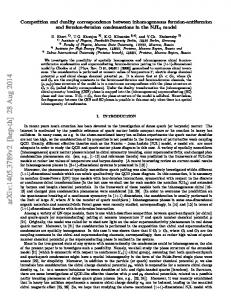
Figure 4. (Top) Plots of hx2 (t)i, comparing real dynamics (symbols) and effective dynamics (solid lines). The dashed lines show the power law scaling of (8), with unit prefactors (we plot hx2 i = t2/(1+µ) ). The effective dynamics captures the timedependence of the mean-squared displacement quantitatively, even at the relatively small value µ = 3. (Bottom) We show the disorder-averaged diffusion front Gn (t) for real dynamics (points) and effective dynamics (lines) at µ = 10 (left) and µ = 3 (right). The times are those of the final points in the top panel, t = 249 and t = 222 : the data of that panel indicate that these times are long enough to be representative of the asymptotic large-time scaling. The effective dynamics agrees well with the real dynamics for µ = 10, but for the smaller µ the agreement deteriorates because the assumption of well-separated time scales breaks down.

In Fig. 4, we compare the predictions of the effective dynamics with simulations of the trap and barrier models. At long times, we find good quantitative agreement at µ = 10. At µ = 3, the effective dynamics still captures the width of the distribution, although the absence of well-separated time scales leads to deviations in the tail. The diffusion front for the trap model was considered in [25], where it was predicted to decay as Gn (t) ∼ |n|(−µ+1)/2µ exp[−b|n|(µ+1)/µ ], for large n and µ close to unity (in our notation, the parameter µ of [25] is denoted by 1/µ). While our results are consistent with this prediction, our statistics are not good enough to accurately determine the asymptotic scaling of the tails of the diffusion front. Overall, we would argue that our results indicate that the proposed effective dynamics does indeed capture the physical processes responsible for propagation in the trap and barrier models.


13

5. Conclusions We have discussed several implications of the duality between one-dimensional trap and barrier models, including (5), which is an exact local relation between their diffusion fronts valid for fixed disorder, and (10), which states that their disorder-averaged propagators are equal. In addition, we have presented a unified effective dynamics for diffusion fronts in the large µ limit of the trap and barrier models. This dynamics captures the scaling of the diffusion front, and gives good quantitative estimates of its width. Our arguments indicate that it gives the exact shape of the diffusion front in the limit of extreme subdiffusion (µ → ∞), with agreement becoming less good as the system approaches the diffusive regime (µ < 1). The effective dynamics exploits the fact that in both models, the time scale on which traps and barriers become irrelevant depend on both their rates W , and on the spacings between them. In the barrier model, the dependence on spacings arises from the fact that if the relevant barriers are well-separated, the particle spends only a small fraction of its time adjacent to them. In the trap model, it originates from the fact that a particle leaving a given trap is likely to be reabsorbed there before it can reach a neighbouring deep trap. Despite the different physical mechanisms, these two processes affect the diffusion front in closely related ways, and mathematically result in the master operators for these processes having equal eigenspectra. Thus, for the purposes of the diffusion front, it is indeed appropriate to consider the barrier model as representing an environment of effective traps in which a particle diffuses. However, as we discussed, the trajectories by which the system evolves in each case are different. The effective dynamics illustrates the nature of these trajectories: in the barrier model, the particle diffuses rapidly within its effective trap, leading to a number of hops growing as N ∼ t. In the trap model, the particle is localised in deep traps, making excursions from its current trap which mostly lead to reabsorption within that trap. The mean hopping rate decreases with time as the system ages [20], leading to N ∼ t2/z . It would be illuminating to investigate whether the duality relation (5) at fixed disorder can be cast as a relation between the particle trajectories in the barrier and trap models, to see whether these different scalings emerge naturally. Given the different physical processes underlying the dynamics of the models, we argue that the relationships between the diffusion fronts are, to a certain extent, coincidental. They do not represent a physical equivalence of the models themselves, and they do not generalise in a simple way to correlation functions other than the diffusion front. However, it seems to us that the equality of the disorder-averaged propagators and the associated algebraic structure might be exploited in further analytic work on these models.


14

Acknowledgments We thank Peter Mayer for very helpful discussions. RLJ was funded initially by NSF grant CHE-0543158 and later by Office of Naval Research Grant No. N00014-07-1-0689. References [1] M. D. Ediger, Annu. Rev. Phys. Chem. 51, 99 (2000); E. R. Weeks et al., Science 287, 627 (2000); W. Kegel and A. van Blaaderen, Science 287, 290 (2000). [2] M. T. Cicerone, P. A. Wagner, and M. D. Ediger, J. Phys. Chem. B 101, 8727 (1997); R. Yamamoto and A. Onuki, Phys. Rev. Lett. 81, 4915 (1998); C. Donati et al., Phys. Rev. E 60, 3107 (1999); B. Doliwa and A. Heuer, Phys. Rev. E 67, 030501 (2003); Y. Jung, J. P. Garrahan and D. Chandler, Phys. Rev. E 69, 061205 (2004). [3] See, for example, M. J. Saxton and K. Jacobson, Annu. Rev. Biophys. Biomol. Struct. 26, 373 (1997); M. Weiss et al., Biophys. J. 87, 3518 (2004); D. S. Banks and C. Fradin, Biophys. J. 89, 2960 (2005); I. Golding and E. Cox, Phys. Rev. Lett. 96, 098102 (2006); M. A. Lomholt, I. M. Zaid and R. Metzler, Phys. Rev. Lett. 98, 200603 (2006). [4] J. Bernasconi et al., Phys. Rev. Lett. 42, 819 (1979). [5] S. Alexander et al., Rev. Mod. Phys. 53, 175 (1981). [6] S. Havlin and D. Ben Avraham, Adv. Phys. 36, 695 (1987). [7] J.-P. Bouchaud and A. Georges, Phys Rep 195, 127 (1990). [8] R. Metzler and J. Klafter, Phys. Rep. 339, 1, (2000). [9] X. H. Qiu and M. D. Ediger, J. Phys. Chem. B 107, 459 (2003). [10] C. Dalle-Ferrier et al., Phys. Rev. E 76, 041510 (2007). [11] L. Davison, D. Sherrington, J. P. Garrahan and A. Buhot, J. Phys. A, 34, 5147 (2001). [12] J. P. Garrahan and D. Chandler, Proc. Nat. Acad. Sci. USA 100, 9710 (2003). [13] For a review, see F. Ritort and P. Sollich, Adv. Phys. 52, 219 (2003). [14] Subdiffusive propagation is characterised by a dynamical exponent z, which describes the relative scaling of space and time at a critical point. For example, the fragile models considered in [15] exhibit subdiffusive behaviour, with z > 2. In the Fredrickson-Andersen model considered in [16], the scaling at the critical point is diffusive, with z = 2. Away from criticality, the correlation length ξ and correlation time τ satisfy Dτ ∼ ξ 2 , where D is the diffusion constant. However, D itself has a non-trivial temperature dependence, so the temperature scaling cannot in general be written as τ ∼ ξ 2 . [15] S. Whitelam and J. P. Garrahan, Phys. Rev. E 70, 046129 (2004); L. Berthier and J. P. Garrahan, J. Phys. Chem. B 109, 3578 (2005). [16] G. H. Fredrickson and H. C. Andersen, Phys. Rev. Lett. 53, 1244 (1984); S. Whitelam, L. Berthier and J. P. Garrahan, Phys. Rev. Lett. 92, 185705 (2004); R. L. Jack, P. Mayer and P. Sollich, J. Stat. Mech. (2006) P03006; P. Mayer and P. Sollich, J. Phys. A 40, 5823 (2007). [17] E. Bertin, J.-P. Bouchaud and F. Lequeux, Phys. Rev. Lett. 95, 015702 (2005). [18] F. Dyson, Phys. Rev. 92, 1331 (1953). [19] P. le Doussal, C. Monthus and D. S. Fisher, Phys. Rev. E 59, 4795 (1999) [20] C. Monthus and J.-P. Bouchaud, J. Phys. A 29, 3847 (1996). [21] J. Machta, J. Phys. A 18, L531 (1985) PM T [22] To see this, use (1) to obtain (d/dt) n=N (xn − xk )GT n←k (t) = (xM − xN )[WN GN ←k (t) − T WM GM←k (t)]. Taking site M far to the right of site k, and site N far to its left, this time P derivative vanishes. Therefore, using the initial condition for GT , we have n (xn −xk )GT n←k (t) = P T ′ T ′ ′ ′ 0. Hence, h[x(t) − x(t )]x(t )i = nk (xn − xk )xk Gn←k (t − t )Gn←i (t ) = 0. [23] C. Monthus, Phys Rev E 68, 036114 (2003). [24] C. Monthus, Phys Rev E 69, 026103 (2004).

Duality between random trap and barrier models [25] E. Bertin and J.-P. Bouchaud, Phys. Rev. E 67, 026128 (2003).

15