➠
➡ DWT-BASED PHONETIC GROUPS CLASSIFICATION USING NEURAL NETWORKS Pham Van Tuan and Gernot Kubin Signal Processing and Speech Communication Laboratory University of Technology, Graz, Austria
[email protected] ;
[email protected] ABSTRACT
2. ADVANTAGES OF DWT IN SPEECH PROCESSING
This paper presents an improvement of the Discrete Wavelet Transform (DWT)-based phonetic classification algorithm by using Neural Networks (NN) to learn optimal thresholds for speech classification. Two feedforward NNs (two layers) operate on input features extracted from speech frames (10ms length) by DWT and statistical measurement in order to classify these frames as transient, voiced vowel, voiced consonant and unvoiced consonant categories. Hard thresholds in our earlier paper are used to detect silence and voiced closure intervals. The new algorithm is tested with the TIMIT database and compared with other algorithms to demonstrate its superior performance. 1. INTRODUCTION The classification of speech frames is an important step in many speech processing applications. Some speech coding systems require phonetic classification to determine the optimal bit allocation for every different speech frame. The discrimination between phonetic classes will improve quality and performance of data-driver speech synthesizers. Speech classification has been studied by a variety of methods. Some linear speech classification such as [7] use statistical features (relative energy level, zero crossing rate,etc) of the speech signal to decide about voiced, unvoiced or silence. In other approaches, the specific spectral charactersitic of speech sounds are exploited by optimal filters designed to discriminate among speech classes [3]. Furthermore, some DWT-based algorithms have been developed to achieve classification at the phonetic level [1],[2]. Since the development of the backpropagation learning algorithm, the feedforward NN has been used widely in pattern recognition and, in particular, for speech classification with promising potential [4], [5], [6]. In this paper, we propose a new combined system of linear and NN-based nonlinear classifiers using wavelet parameters as well as statistical parameters to increase the performance and robustness of an optimal threshold-based speech classifier. The goal is to classify 10ms speech frames into phonetic categories [1]. Then, smoothing and interpolation techniques are used to mark boundaries between phonetic groups which we define as homogeneous sequences of speech sounds that belong to the five phonetic classes considered above. One of our new contribution is the consideration of so-called ”wavelet-detail ratio features” across two neighbouring frames as input for the transient detection. Gender-dependent and gender-independent NN classifiers are built to study and evaluate the impact of speaker dependency on speech classification.
0-7803-8874-7/05/$20.00 ©2005 IEEE
Any signal s(t) can be represented with basic functions as: XX dm,n ψm,n (t) s(t) = m
(1)
n
−m/2
ψ(a−m t − nb0 ) are basis functions and where ψm,n (t) = a0 0 dm,n are the coefficients of the DWT of s(t) for all m, n ∈ Z, Z ∞ −m/2 dm,n = a0 s(t)ψ(a−m − nb0 )dt (2) 0 −∞
With a0 = 2 and b0 = 1, we obtain the dyadic DWT. The advantage of DWT in speech processing is based on the relation between DWT and multiresolution analysis (MRA) which provides the structure for a multiscale decomposition of a signal. If we have a function s(t), it can be decomposed into the sum of a low-pass approximation plus L details at L resolution stages as: s(t) =
∞ X
cL,n 2−L/2 φ(
n=−∞ L ∞ X X
−m/2
dm,n 2
m=1 n=−∞
t − n)+ 2L
(3)
t ψ( m − n) 2
where φ(t) and ψ(t) are a scaling function and a wavelet function, cm,n and dm,n are the approximation or scaling coefficients (low-frequency part) and the detail or wavelet coefficients (highfrequency part) of the output of the DWT which are given by: cm,n =
∞ √ X 2 cm−1,k h0 (k − 2n)
(4)
k=−∞
dm,n =
√
2
∞ X
cm−1,k h1 (k − 2n)
(5)
k=−∞
where h0 (n) and h1 (n) are synthesis low-pass and high-pass responses of a two-band paraunitary filter bank. Typically, the energy of the voiced vowel frames is mostly contained in the approximation part and much less in the detail part and vice verse for the unvoiced consonant frames. The relative equal energy distribution occurs in the voiced consonant frames. So, this property can be used in the specific representation of the three different classes. Furthermore, the signal is decomposed into different scale levels, and the energy of the details varies over different scales in different ways, depending on the input signal (a
I - 401
ICASSP 2005
➡
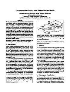
➡ property similar to spectral tilt). We observe this energy variation of the detail coefficients for voiced vowel frames in Fig. 1-a and unvoiced consonant frames in Fig. 1-b as:
As the basis for the phonetic classifier, we need to extract the following representative features from each frame which has 10ms length corresponding with K=160 samples:
E(d1,n ) < E(d2,n ) < E(d3,n ) < E(d4,n )
(6)
E(d1,n ) > E(d2,n ) > E(d3,n ) > E(d4,n )
(7)
• Approximation wavelet energy ratio (AWER) is the ratio of the energy in the approximation coefficients and the energy of all wavelet coefficients at the first level of wavelet analysis: PN1 2 n=1 (c1 ,n ) (8) AW ER = PN1 P 2 N1 2 n=1 (c1 ,n ) + n=1 (d1 ,n )
A voiced segment of 10ms length
1
−1
An unvoiced segment of 10ms length
0.5
0
0 20
40
60
80
100
120
140
160
−0.5
20
Detail coefficients of DWT Level
Level
2 3 20
dB
60
80
100
120
140
160
where c1,n and d1,n are the approximation and detail coefficients (length N1 ) at the first level wavelet analysis.
2 3 4
4 40
60
80
100
120
Power spectral density
140
20
160
samples
40
60
80
100
120
Power spectral density
140
160
samples
• The energy variation of detail coefficient (EVD), (see Fig. 1) is defined by the following equation:
−50
dB
−40 −60 −80 0
40
Detail coefficients of DWT
1
1
1000
2000
3000
4000
5000
6000
7000
8000
Hz
−100 0
1000
(a) voiced frame
2000
3000
4000
5000
6000
7000
Hz
8000
(b) unvoiced frame
Fig. 1: Energy variation of detail coefficients over 4 levels and power spectral density From the observation at the first three levels of wavelet analysis in Fig. 2, we can also apply the energy variation of detail coefficients for transient classification when considering two neighboring frames. A transient frame always has higher absolute energy in its details coefficients than a closure interval frame which may be silence or periodic. This characteristic is used to define the closure interval-transient detail energy ratio and combining with other statistical features to detect transient frames. 0.2
Closure Interval and Transient frames
• The closure interval-transient detail ratio (CTDR) is the ratio of the detail coefficient energies at the same wavelet analysis level, computed for the closure interval and the following transient frame in Fig. 2: PNm 2 (dm,n )2 CT DR(m) = Pn=1 (10) Nm 1 2 n=1 (dm,n ) where d1m,n and d2m,n are the wavelet detail coefficients of the closure interval and the transient frame, Nm is the length of the sequences d1m,n and d2m,n .
0 −0.1 50
100
150
200
250
• Short-term average energy (SAE) is calculated for each frame:
300
Detail coefficients of DWT
Level
1
20 40
SAE =
60
2
80 100
3
120
50
100
150
200
250
(9)
where Nm and Nk are lengths of detail coefficient sequences dm,n and dk,n at different analysis level m and k.
0.1
−0.2
Nk Nm 1 X 1 X (dk ,n )2 (dm ,n )2 − Nm n=1 Nk n=1
EV D(m, k) =
K 1 X s(i) 2 · ( ) K i=1 sp
(11)
300
where s(i) are the samples of 10ms frame, and sp is the peak value of the input signal.
time (samples)
Fig. 2: Different energy variation of detail coefficients over first 3 levels for a closure interval followed by a transient frame. 3. FEATURE EXTRACTION
• Zero crossing rate (ZCR) is a measure of frequency content of each speech frame:
As discussed in the introduction, we want to classify five types of phonetic groups which are homogeneous frames sequences having the same phonetic characteristics as follows: ∗ A silence group are frames which have a very low overall amplitude level and a blank spectrogram. ∗ A voiced vowel group includes vowels, semivowels and diphthongs which have a repetitive time-domain structure and lowfrequency voiced striations in the spectrogram. ∗ A voiced consonant group includes voiced and glottal fricatives which have both periodic and noise-like properties, and nasals, which have a weak and interrupted voice bar in the spectrogram. ∗ An unvoiced consonant group includes only unvoiced fricatives which have an irregular time-domain structure and only high frequencies in the spectrogram. ∗ A transient group include plosives and affricates which contain a transient frame inside.
ZCR =
K X
|sgn[s(i) − sgn(s(i − 1))]|
(12)
i=1
4. NEURAL NETWORK CLASSIFIER 4.1. Network configuration setup A supervised learning algorithm is used to train a two-layer feedforward network. This means that the network weights and biases are adjusted to minimize the mean square error between the network outputs and real target outputs. We train a first network with 5-dimensional input vectors and 1dimensional output to detect transient frames. Second network is configured with 4-dimensional input vectors and 3-dimensional output to perform the three-way classification: voiced vowel frame, voiced consonant frame and unvoiced consonant frame. The output is labeled as 1 for the desired frames and 0 for other frames.
I - 402
➡
➡ As a preprocessing step, all elements of the input and output vectors are normalized to get zero mean and unity standard deviation over the training set. The feedforward networks use log-sigmoid transfer functions for all hidden units in their hidden layer and linear transfer functions at the output layer. Biases and weights of each unit are initialized to very small random values.
units nH, which achieves the lowest error percentage on the training and test sets of the one-class NN classifier and three-classes NN classifier for female speaker is 0.75 − 60 and 0.40 − 100 (Fig. 3-b), for male speaker is 0.55 − 55 and 0.50 − 125, and for mixedspeaker is 0.55 − 70 and 0.65 − 110. 5. COMBINED CLASSIFICATION ALGORITHM
4.2. Network learning algorithms To avoid overfitting in the backpropagation learning algorithm, a weight decay heuristic (regularization) is used to decrease each weight by some small factor during each iteration. This modifies the typical performance function by adding a penalty term corresponding to the sum of squares of the network weights [9]:
• The number of iterations epochs = 1000. • The training performance goal = 1e − 5 • The performance ratio and the number of hidden units are varied as γ = [0.3, 0.35, ..., 0.8] and nH = [5, 10, ..., 140] to find out the optimal values where the sum of training and testing error rate is smallest. The datasets are taken from the TIMIT database, dialect speaking region 1 (DR1). Each dataset is divided into 70% training set and 30% test set. Female speaker and male speaker datasets are collected separately to investigate a gender-dependency of the phonetic classifier. Another mixed dataset containing both of genders is used to design a gender-independency phonetic classifier. 8.5
Classification Error Rate (%)
Classification error rate (%)
9
Levenberg−Marquardt BFGS Quasi−Newton Adaptive Learning Rate Adaptive Learning Rate + Momentum
10
7.5
9 8
7
6.5
7 6
6
5.5
5 4 0
Train − ratio=0.4 Test − ratio=0.4 Train − ratio=0.6 Test − ratio=0.6
8
5
20
40
60
80
100
120
Number of hidden units in their hidden layer
(a) the best learning algorithm at γ = 0.5
140
4.5 0
20
40
60
80
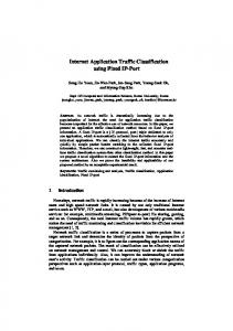
The 1st NN Classifier
True
False
Transient ?
True
Interpolation & Smoothing
False
• The learning rate lr = 0.05.
11
Silence/voiced closure interval ?
Linear Classifier
(13)
where γ is a performance ratio, wj are the weights of the NN, and ti and oi are the output and target values, respectively. This approach results in smaller weights and biases and forces the network response to be smoother over its complex decision surface [8]. We select the best learning algorithm among the following ones: momentum, variable learning rate, Levenberg-Marquardt and BFGS Quasi-Newton algorithms. Some common parameters of the learning algorithms are set as follows:
12
Speech features
Presmoothing
N M 1 X 1 X (ti − oi )2 + (1 − γ) (wj )2 Ereg = γ N i=1 M j=1
13
A phonetic group classification algorithm is proposed with four sequential steps shown in Fig. 4.
100
120
140
Number of hidden units in their hidden layer
(b) the best performance ratios for LM algorithm
Fig. 3: The average error percentage on the training set and the test sets for the three-classes NN classifier and for female speaker. From the results of the training phase, we see that the Levenberg Marquardt (LM) algorithm gives the highest classification performance generally (Fig. 3-a). For this learning algorithm, the optimal choice of the performance ratio γ and number of the hidden
Final Decision
Voiced vowel/ Unvoiced consonant/ Voiced consonant
The 2nd NN Classifier
Fig. 4: The classification combined algorithm. • First, silence (S) and voiced closure interval frames are detected by linear classifier (see Fig. 5) using threshold-based decision model in [1], with AW ER3 = 99%, EV D1 = 0.15, EV D2 = 0.35, SAE1 = 0.001/160, SAE2 = 0.025/160 and SAE3 = 0.016/160 (where SAE3 is a new threshold suggested to improve silence detection). Subsequently, presmoothing is used to eleminate some wrong decisions to decrease probability that the transient classifier can make incorrect decisions. Speech features False
SAE