DYNABYTE: A Dynamic Sampling Algorithm for Redundant Content ...

DYNABYTE: A Dynamic Sampling Algorithm for Redundant Content Detection Emir Halepovic, Carey Williamson and Majid Ghaderi Department of Computer Science University of Calgary 2500 University Drive NW, Calgary, AB, Canada T2N 1N4 {emirh, carey, mghaderi}@cpsc.ucalgary.ca Abstract—Protocol-independent redundant traffic elimination (RTE) is an "on the fly" method for detecting and removing redundant chunks of data from network-layer packets traversing a constrained link or path. Efficient algorithms are needed to sample data chunks and detect redundancy, so that RTE does not hinder network throughput. A recently proposed static algorithm samples chunks based on highly-redundant trigger bytes observed in data content. While this algorithm is fast, it requires pre-computed traffic information for the configuration of its static parameters, and it tends to either under-sample (reducing byte savings) or over-sample (increasing processing cost) on heterogeneous traffic. We propose a dynamic sampling algorithm for redundant content detection. Our algorithm is adaptive and self-configuring, and can precisely match the specified sampling rate. Furthermore, it offers byte savings comparable to the static algorithm, with very low additional processing overhead. Keywords-Algorithm, Sampling, Redundancy, Elimination, Performance, Network, Traffic

Detection,

I. INTRODUCTION Redundancy detection is widely used in the storage, management, and transmission of digital content. Example applications include file compression [12], data de-duplication in storage systems [6], plagiarism detection [10], and redundant traffic elimination (RTE) in networks [1, 2, 11]. Algorithms for redundancy detection generally involve a sampling stage to establish suitable "fingerprints" for content, and a matching stage to compare new samples to those that have been seen previously. In some applications, an additional stage is used to encode the redundant content in a compact form, or decode it to restore the original data. The sampling and fingerprinting stage typically incurs the highest processing cost, necessitating an efficient algorithm [1]. This consideration is especially important for RTE, which needs to operate at link speed, without hindering throughput. The observed redundancy in Internet data traffic is typically 15-60% [2]. This redundancy arises from the skewed popularity of content [3, 4], leading to repeated transfers of popular content to many users. Transfers of redundant content can waste network resources, saturate limited-bandwidth links (e.g., wireless or cellular access networks), and increase economic costs for users (e.g., usage-based charges). The most obvious approach to redundancy elimination is object-level caching, which is widely used in Web caches,

proxies, and content delivery networks. However, these approaches are not as effective as protocol-independent RTE at the IP-layer [11]. RTE relies upon middle-boxes inserted at two ends of a bandwidth-constrained link. An RTE module runs on each of these middle-boxes and maintains a cache of recently transferred packets. When a new arriving packet carries data that matches content in the cache, the packet is encoded using fewer bytes and transferred across the bandwidth-constrained link. The RTE module at the other end of the link decodes the data and reconstructs the original packet. This technique captures redundancy inside and across objects, and is also protocol-independent. A recent proposal advocates RTE at end-systems rather than inside the network [1]. To support this approach, a new sampling algorithm, SAMPLEBYTE, was designed that can run on end-user devices such as mobile phones [1]. SAMPLEBYTE provides efficient execution, with adjustable processing cost. The latter feature is important on batterypowered devices, since the sampling rate of the algorithm directly affects processing costs. While SAMPLEBYTE is simple, efficient, and performs well with suitable settings for chunk size and sampling period, it requires pre-configuration based on training data. Furthermore, its configuration remains static throughout operation. In this paper, we study the sensitivity, robustness, and performance of SAMPLEBYTE under other parameter configurations, specifically with larger chunk size and sampling period. In addition, we study if the benefits of SAMPLEBYTE can be achieved in a dynamic manner, without training. In particular, we propose a self-configuring dynamic algorithm, DYNABYTE, as a logical extension of SAMPLEBYTE, and show that it achieves comparable byte savings to SAMPLEBYTE. DYNABYTE improves upon the sampling heuristic, providing precise control of the sampling rate, predictable processing cost, and low overhead compared to the static configuration. The rest of this paper is organized as follows. Section II reviews prior related work. Section III describes the data sets and methodology used. Section IV provides an overview of SAMPLEBYTE, with detailed analysis following in Section V. Section VI presents the new DYNABYTE algorithm, while Section VII provides the evaluation results. Section VII concludes the paper.

Distance

Skip

Overlap

TABLE 1: SUMMARY OF THE DATA TRACES (GB)

Payload Chunk A

Chunk B

Marker FP B = fingerprint (Chunk B)

Chunk C FP A

Chunk A

FP B

Chunk B

Chunk cache

Fig. 1: Terminology of RTE.

II. BACKGROUND AND RELATED WORK Content-based chunking is the most general technique for redundancy elimination. Objects or files are divided into chunks, with comparison between chunks made within or across files (Fig. 1). The first byte of each chunk is called a marker. Chunks generally do not correspond to a specific location inside the file. Rather, they are defined by their content, so they may overlap, or have some distance between them. Data chunks can have a fixed or varying size. Chunks are identified using a probabilistically unique hash value called a fingerprint. Fingerprints are commonly SHA-1 checksums or Rabin fingerprints [6, 8, 11]. Rabin fingerprints are especially useful because they can be computed efficiently using a sliding window over a byte stream. Fingerprints and chunks are stored in a chunk cache or packet cache, in case of RTE, at two ends of the network link or path. Depending on the implementation, chunks may not need to be stored in the sender side cache, but fingerprints are always stored. The receiver side normally stores both fingerprints and chunks. When a redundant chunk is identified using a fingerprint on the sender side, instead of sending the whole chunk, only meta-data is sent. The encoded meta-data may consist of fingerprints or other information sufficient to reconstruct the whole chunk or a matching region using the receiver-side cache. In some cases, the matched region can be expanded beyond the identified chunk to increase the detected redundancy. In some RTE systems, the caches at each endpoint must be synchronized to contain information about the same packets and chunks [1, 11], while in others, they do not [9]. The original proposal envisioned caches to be placed at the ends of a constrained link inside the network [11]. Today, high-end hardware products using RTE are deployed between geographically distributed offices of a single enterprise [5]. This approach is often called WAN optimization. Regardless of the architecture or particular deployment, the core of any RTE engine is a sampling algorithm. A fraction 1/‫ ݌‬of all possible chunks is selected for caching, since it is impractical to cache all possible chunks. The parameter p (e.g., ‫ = ݌‬32) is called the sampling period. The selection of chunks is based on some property of either the chunk or its fingerprint, such as its numeric value [2] or a specific byte pattern [11].

Trace

Date

Time

In

Out

Total

1 2 3 4 5 6 7 8

April 6, 2006 April 6, 2006 April 7, 2006 April 7, 2006 April 8, 2006 April 8, 2006 April 9, 2006 April 9, 2006

9 am 9 pm 9 am 9 pm 9 am 9 pm 9 am 9 pm

19.9 8.2 23.6 18.3 8.8 18.9 7.7 21.9

15.5 14.9 16.9 12.5 8.2 12.3 10.6 15.4

35.4 23.1 40.5 30.8 17.0 31.2 18.3 37.3

TABLE 2: APPLICATION PROFILE FOR CAMPUS TRACES Direction

HTTP

Email

Inbound Outbound

45% 30%

7% 6%

P2P

SSL

Other

Unknown

11% 23%

9% 7%

6% 7%

22% 27%

III. DATA SETS AND METHODOLOGY In this paper, we use full-payload network traces collected from the Internet access link at the University of Calgary. A total of 8 traces were collected, each one hour in duration, starting at 9 am and 9 pm each day. All traces are bidirectional. The total IP payload transmitted is 233.6 GB. The details of each trace are shown in Table 1. These traces complement the campus data set used in previous work [2]. We further divide traces into incoming and outgoing traffic, which are studied separately. The main reason for this is that different levels of redundancy may exist in each direction. The volume of data traversing different directions may also call for different cache sizes, RTE algorithms, or parameters. We show the application profile of inbound and outbound traffic for the aggregate traces in Table 2. Our traces have similar composition as the one analyzed in [2]. A custom-written simulator is used for the evaluation of the algorithms. Simulations are performed on a Linux-based server with 3 GHz quad-core CPU, and 32 GB of RAM. Our primary metrics for evaluation are byte savings, processing time, and actual sampling rate. We use 64-byte chunks with a range of sampling periods. The byte savings represent net savings after including an encoding overhead penalty of 5 bytes per chunk. When using fixed-size chunks, we only need to encode the chunk location in the packet payload, and the offset in the cache. The location within the packet payload can be encoded with 11 bits, and a 512 MB cache can store 8 million 64-byte chunks. Therefore, we need a total of 11 + 23 = 34 bits of overhead per chunk. For larger caches, or any additional meta-data, increasing the penalty to 40 bits (5 bytes) per chunk still represents only 7.8% overhead for the 64-byte chunk. Smaller chunk sizes would have correspondingly higher overhead, since more chunks could be stored in the cache.

1 2 3 4 5 6 7 8 9 10

//Let w = 32; p = 32; Assume len >= w; //TABLE[i] maps byte i to either 0 or 1 //hash() computes a hash over a w byte window SAMPLEBYTE(data, len) for(i = 0; i < len - w; i++) if (TABLE[data[i]] == 1) marker = i; fingerprint = hash(data + i); store marker, fingerprint in cache; i = i + p/2; Fig. 2: SAMPLEBYTE algorithm.

IV. OVERVIEW OF SAMPLEBYTE SAMPLEBYTE combines the robustness of content-based sampling with the computational efficiency of fixed selection (Fig. 2) [1]. Content-based sampling is robust against small changes in object content, and fixed selection is very fast, since it computes fingerprints for exactly 1/‫ ݌‬sampled chunks at regular fixed locations. SAMPLEBYTE uses a 256-entry lookup table, with one entry for each possible byte value. A fixed set of k byte values are specified as markers and they trigger chunk selection. As a data block is scanned byte-by-byte (line 5 in Fig. 2), a byte is chosen as a chunk marker if the corresponding entry in the lookup table is set (lines 6 and 7). A fingerprint is then computed using Jenkins Hash (line 8) and ‫݌‬/2 bytes of content are skipped (line 10) before the sampling process resumes. The special marker bytes are set by using a training trace with an algorithm that does not depend on byte frequencies [10]. The most prevalent redundant bytes detected in this phase become marker bytes for SAMPLEBYTE, which increases the probability of selecting the most redundant chunks. Clearly, higher k leads to a higher sampling rate, while lower k leads to fewer sampled chunks. In prior work, using ݇ = 8 marker bytes is found to be effective, with negligible improvement in savings when more than 8 marker bytes are used. The identified marker bytes are 0, 32, 48, 101, 105, 115, 116, and 255. We refer to these bytes as "generic markers". Since marker bytes have high redundancy, the top 8 of them can account for 10-12% of all traffic, such as in our traces. Therefore, on average 1 out of every 8-10 bytes will be selected as chunk marker, with high probability, which is much more than expected with ‫ = ݌‬32, for example. The skip parameter is used to limit the worst-case sampling rate, and it is statically configured to ‫݌‬/2 in SAMPLEBYTE. This means that the upper bound is 2/‫݌‬, twice the target rate of 1/‫݌‬. Under-sampling can still happen, since highly redundant bytes, such as 0, 32 (space character), and 255, are often found in consecutive blocks, so many of them are skipped. In previous work, an additional step is used with the goal of increasing the detected redundancy. After a redundant chunk is detected for caching, the matching region is expanded byte by byte around the chunk to achieve the largest possible match [2, 11]. Expansion introduces overhead in processing cost and storage, but improves average detected redundancy by 13.6% over an exact chunk match [1].

We implement SAMPLEBYTE with two modifications. Instead of Jenkins Hash, we use FNV Hash function [7]. In addition, we are interested in a scenario where fixed-size chunks are used for redundancy elimination, instead of expanding the matching region around the selected chunk. These modifications do not affect the relative comparison of algorithms in our work. The key benefits of SAMPLEBYTE are: •

Speed and efficiency. Skipping half of a sampling period avoids unnecessary fingerprint computation for chunks that would not be selected anyway.

•

Bounded sampling rate. The skip parameter limits the maximum sampling rate to 2/‫݌‬. Adjusting p affects the upper bound on sampling rate, which directly determines processing cost.

•

Simpler computation. In a client-server scenario, fingerprint computation is only required at the server. Clients can always determine where chunks start based on the generic markers.

In prior work, SAMPLEBYTE was evaluated on a large set of traces from several enterprises and a university, using default chunk size of 32 bytes and sampling period of ‫ = ݌‬32 [1]. Its performance was found to be satisfactory. We examine if SAMPLEBYTE performs equally well on aggregate traces from multiple users and under different parameters, such as a larger chunks size of 64 bytes, and longer sampling periods, such as 48, 64 or more. The goal of this study is to explore whether a dynamic algorithm can match or exceed the savings of static SAMPLEBYTE at acceptable cost. In particular, we explore the following specific questions about SAMPLEBYTE: •

Are generic marker bytes suitable? As traffic changes, the k generic markers may no longer be the most frequent bytes, which may adversely affect savings or processing time. In other words, generic markers may or may not be representative of the upcoming traffic traversing the link.

•

How many marker bytes are appropriate? In SAMPLEBYTE, the value of k is fixed at 8. While 8 was appropriate for SAMPLEBYTE on a certain set of traces, we would like to ascertain if this holds for our traces. Since k affects sampling rate and savings, we may be over-sampling or under-sampling if we use the wrong number of marker bytes.

•

Is the actual sampling rate predictable? Due to probabilistic sampling based on generic markers, we suspect that the actual sampling rate may deviate substantially from the target 1/‫݌‬. We would like to verify if this happens, and under what conditions. This is especially important if RTE is deployed on a batterypowered device and it needs to control its processing requirements precisely.

V. ANALYSIS OF SAMPLEBYTE To answer our first question, we apply SAMPLEBYTE with 8 generic markers to our traces, and compare its

15%

15%

10%

Sampling rate (%)

b)

a) Specific markers Generic markers

5% 0% 7% 6% 5% 4% 3% 2% 1% 0%

Savings (%)

20%

16

24

32

48 64 Sampling period p

96

128

32

48 64 Sampling period p

96

Next we examine whether ݇ = 8 is an appropriate choice for our traces. We apply SAMPLEBYTE with ‫ = ݌‬32 to one of our traces, using specific markers, and vary k from 1 to 16. We track byte savings, actual sampling rate, and processing time for inbound Trace 2 from our data sets. Fig. 4a shows the increase in savings as k changes. One could reasonably conclude that there are no gains in savings beyond ݇ = 8, but the same argument can be made for ݇ = 6, where the savings plateau. For the generic markers, the savings also reach their maximum at ݇ = 6, though the overall savings are lower by 38%. These results show that there is a benefit to finding the proper k value for each trace. We also notice that the actual sampling rate is well below the target rate for smaller k values, while the opposite happens for larger k values (Fig. 4b). Therefore, while the maximum sampling rate is bounded, it certainly does not closely follow the target rate for any k other than 8. The processing time curve mimics as expected (Fig. 4c), and shows the larger k values. A small increase in increase in processing cost, with no

that for sampling rate, consequence of using k may cause a large improvement in byte

2

3

4

5

6

Time (x1000s)

c)

7 8 9 10 11 12 13 14 15 16 Number of markers k

4% 3% 2%

Target rate

1%

Actual rate 1

2

3

4

5

6

7 8 9 10 11 12 13 14 15 16 Number of markers k

1

2

3

4

5

6

7 8 9 10 11 12 13 14 15 16 Number of markers k

2.0

Fig. 3: SAMPLEBYTE with specific markers vs. generic markers.

Fig. 3 shows the total byte savings and overall sampling rate for inbound Trace 2. (Note that the x-axis is not linear). Specific markers clearly outperform generic markers in savings for all sampling periods, by 24-56% (Fig. 3a). The plot of actual sampling rate shows that both sets of markers result in similar sampling (Fig. 3b). Therefore, the higher savings with specific markers are due to better markers, and not due to a higher sampling rate. This result is a strong argument in favour of traffic-specific markers.

1

5%

0%

128

performance to SAMPLEBYTE using traffic-specific markers ("specific markers"). The top 8 specific markers are obtained from a training trace in the same manner that the generic markers were obtained in [1]. We use a wide range of sampling periods to better illustrate algorithm behaviour, while noting that the important range is between 32 and 64, for commonly used chunk sizes of 32-64 bytes in commercial RTE systems.

Generic markers

6%

b)

24

Specific markers

5% 0%

Specific markers Generic markers Target rate

16

10%

Sampling rate (%)

Savings (%)

a)

20%

1.5 1.0 0.5 0.0

Fig. 4: SAMPLEBYTE behaviour as number of markers changes.

savings. For example, the savings obtained for ݇ = 6 and ݇ = 8 are the same, while the processing time for ݇ = 8 is 14% higher. Finally, we examine the actual sampling rate across several sampling periods p. We fix k at 8 and repeat the experiment to observe the behaviour of SAMPLEBYTE with generic markers. The results are shown in Fig. 5. The detected redundancy decreases as the sampling period increases, as expected, due to fewer selected chunks (Fig. 5a). Once the encoding penalty is taken into consideration, the net byte savings actually do not change much. Therefore, we may be able to adjust the sampling period in order to control CPU usage, while maintaining similar byte savings. We further note that the actual sampling rate changes only by a factor of 3 when the sampling period varies by a factor of 8 (Fig. 5b). Therefore, there is no direct correspondence between actual sampling rate and given sampling period. SAMPLEBYTE under-samples for smaller p, and oversamples for larger p. Having the actual sampling rate correspond more closely to the given sampling period is desirable. Similarly, it would be desirable if processing time was directly controllable via the sampling period. If we were to sample with ‫ = ݌‬32, and the system is too busy to sustain this value, it may request the RTE process to reduce its load by half. While we might intuitively expect that doubling p to 64 would reduce processing time by 50%, the actual reduction is only 30% in Fig. 5c. When energy is scarce, we would like to make good tradeoffs between savings versus required power. The highest

4/3‫݌‬. In DYNABYTE, we use these two parameters to control the actual sampling rate, while following some basic principles of AIMD (Additive Increase Multiplicative Decrease) control.

20%

a)

Savings (%)

15% 10%

Sampling rate (%)

0%

b)

Redundancy Savings

5%

7% 6% 5% 4% 3% 2% 1% 0%

16

24

32

Time (x1000s)

96

128

Target rate Actual rate

16

24

32

2.0

c)

48 64 Sampling period p

48 64 Sampling period p

96

128

1.5 1.0 0.5 0.0

16

24

32

48 64 Sampling period p

96

128

Fig. 5: SAMPLEBYTE behaviour as sampling period changes.

savings of 12.3% are achieved with ‫ = ݌‬48. If we were to accept a small penalty in savings of 1% (relative), we would reduce processing cost by 15%. For a 7% sacrifice of savings, we could reduce processing cost by 33% with ‫ = ݌‬96. Therefore, there is room for substantial savings in processing time. The presented results show that both savings and processing cost could be improved by specific markers, properly adjusted k, and the precise sampling rate. VI. DYNABYTE: DYNAMIC SAMPLEBYTE... Armed with a better understanding of the benefits and drawbacks of static SAMPLEBYTE, we can now describe the design of DYNABYTE. The goal with DYNABYTE is to preserve the benefits of SAMPLEBYTE, such as byte savings and adjustable processing cost, without requiring any training phase or pre-configuration. We also want precise control of the sampling rate. A. Achieving the target sampling rate To track if the algorithm is matching the target sampling rate, it suffices to count the number of sampled chunks. The actual sampling rate is compared to the target after a suitable interval, e.g. S seconds, or B bytes. The sampling rate can be adjusted using the existing skip and k parameters in SAMPLEBYTE. By changing k, we alter the cumulative probability of the marker bytes, which in turn affects the probability of finding a marker within the next block of bytes. By adjusting skip, we can also change the sampling rate. For example, for ‫ = ݌‬32, increasing skip from 16 to 24 reduces the worst-case sampling rate from 2/‫ ݌‬to

Consider the skip parameter and its range. For ‫݌ = ݌݅݇ݏ‬, the actual sampling rate will be at most 1/p. Therefore, skip should never exceed p, if we are close to the target sampling rate. On the other hand, we should not allow ‫݌ < ݌݅݇ݏ‬/2. The reason for this is that we should avoid selecting chunks that have too many overlapping bytes. For a chunk size of 64 bytes and ‫ = ݌‬32 , ‫݌ = ݌݅݇ݏ‬/2 allows up to 48 bytes of overlap between consecutive chunks. If both chunks are redundant, then the second chunk provides only 16 bytes of detected redundancy. With an encoding penalty of 5 bytes, we save a total of 11 bytes, which is only 17% of the chunk size. Needless to say, these savings are not worthwhile. The important feature of skip is that it precisely bounds the sampling rate within a factor of 2, when in the range [‫݌‬/2, ‫]݌‬. This is why skip is the primary control parameter in DYNABYTE. The k parameter, on the other hand, has a larger range from 1 to 256, and its effect on sampling rate is more difficult to predict. Therefore, we will use k as a secondary control parameter in DYNABYTE. The sampling rate adjustment will be made first by changing skip, and if one of the limits imposed on skip is reached, then k will be adjusted. The initial value for skip is ‫݌‬/2, and for k it is 8. B. Dynamic adjustment of marker bytes To ensure that markers correspond to traffic, we use a simple history-based ranking of bytes. For each interval i, we compute byte frequencies and select the top k bytes as markers for the following interval ݅ + 1. This interval may be the same as the rate-adjusting interval, but does not have to be. We track the changes in the top 8 markers for each 16 MB interval on our training trace, and find that changes are rare, with 1 or 2 bytes changing on most occasions. Therefore, frequent updates of chunk markers are not necessary. C. DYNABYTE algorithm The pseudo-code for DYNABYTE is shown in Fig. 6. The data of length length is scanned byte by byte (line 8). Each scanned byte is checked in the TABLE to see if it is a chunk marker (line 9). If so, the chunk is selected for caching, and its fingerprint is calculated (line 10). If the selected chunk is a cache hit, it is encoded (or decoded) inside the data packet (line 11). Otherwise, the chunk and its fingerprint are added to the cache (line 12). Relevant counters and byte frequencies are also calculated (lines 13 and 14). The chunk_counter variable is used to track the actual sampling rate. Periodically, the algorithm updates the TABLE based on byte frequencies (line 17). It also periodically checks the actual sampling rate (line 19). If the sampling rate is more than a threshold t off target (line 23), parameters are adjusted (lines 25 and 28). The algorithm first adjusts the ‫ ݌݅݇ݏ‬parameter, as required. If ‫ ݌݅݇ݏ‬has reached one of its limits, then the algorithm switches to adjusting ݇ instead (lines 26 and 29).

Savings (%)

a)

70% 60% 50% 40% 30% 20% 10% 0%

b)

Therefore, when correcting over-sampling, skip is adjusted to the maximum value p, which guarantees a sampling rate of at most 1/‫݌‬. In this case, k is immediately reset to its default value of 8. Note that this approach solves the problem of oversampling from a large k (Fig. 4), and obviates the need to find the best k for a particular type of traffic. When under-sampling, skip is adjusted proportionally based on the degree of under-sampling and the available range of values. For example, if ‫ = ݌‬32, then the minimum skip value is ݉݅݊_‫ = ݌݅݇ݏ‬16. Therefore, the available range is (‫ ݌‬− ݉݅݊_‫)݌݅݇ݏ‬. If under-sampling by a factor of m, then the new skip value is calculated as ‫ ݌݅݇ݏ = ݌݅݇ݏ‬− (݉ − ‫ ݌()ݐ‬− ݉݅݊_‫ )݌݅݇ݏ‬, where t is the tolerance threshold. The under-sampling factor is moderated by the tolerance threshold, to avoid excessive adjustment if the threshold was barely exceeded. If skip is already at the smallest allowed value when undersampling by a factor of m, then k needs to be increased. Since the range of k is much larger, increasing k proportionally causes large jumps in sampling rate, which is undesirable. Again, we respond slower to under-sampling than to oversampling. Therefore, we use a slow increase in k as follows: ݇ = ݇ + (݉ − ‫()ݐ‬256 − ݇)/8,

0

500

1000

1500 2000 2500 Processed data (MB)

3000

1500 2000 2500 Processed data (MB)

3000

3500

4000

SAMPLEBYTE DYNABYTE Target rate

5% 4% 3% 2% 1% 0%

0

500

1000

20

3500

4000

15

c)

10

Skip and k

d)

SAMPLEBYTE DYNABYTE

5 0

Fig. 6: DYNABYTE algorithm.

D. Adjusting skip and k Both skip and k may be adjusted in small or large steps. Naturally, both can be adjusted by 1, but this causes a slow response in sampling rate. Most importantly, algorithm should respond rapidly to over-sampling in order to minimize use of CPU and/or battery power.

DYNABYTE SAMPLEBYTE

6%

Sampling rate (%)

// Assume length >= chunk_size; // TABLE[i] maps byte i to either 0 or 1 // hash() computes FNV hash over a w-byte chunk chunk_size = 32; p = 32; chunk_counter = 0; target_r = 1/p; t = 0.05; skip = p/2; k = 8; DYNABYTE(data, length) { for (i = 0; i < length - w; i++) if (TABLE[data[i]] == 1) fingerprint = hash(data + i); if (cache_hit(fingerprint)) encode data else add fingerprint and chunk to cache; chunk_counter++; update_byte_frequencies(chunk); i = i + skip; if (at_table_adjustment_period(i)) adjust_table(); if (at_rate_adjustment_period(i)) adjust_rate(chunk_counter, i) } adjust_rate(counter, processed_data) { actual_r = counter / processed_data; if (actual_r and target_r within t) return; if (actual_r > target_rate) skip = p; k = 8; else if (skip > 1) decrease skip else if (k < 256) increase k; }

Time (s)

1 2 3 4 5 6 7 8 9 10 11 12 13 14 15 16 17 18 19 20 21 22 23 24 25 26 27 28 29 30

36 32 28 24 20 16 12 8 4 0

0

500

1000

1500 2000 2500 Processed data (MB)

3000

3500

4000 skip k

0

500

1000

1500 2000 2500 Processed data (MB)

3000

3500

4000

Fig. 7: Behaviour of SAMPLEBYTE and DYNABYTE per interval.

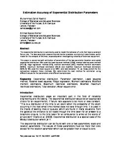
where t is the tolerance threshold. The division by 8 is found to perform well, and causes no abrupt increases in sampling rate. Incrementing k by 1 or 2 would also be acceptable. VII. EVALUATION OF DYNABYTE To evaluate DYNABYTE, we conduct a direct comparison with SAMPLEBYTE. Both algorithms are applied to the full set of our traces, with different sampling periods. To provide the fairest possible comparison, specific markers are used for SAMPLEBYTE, since they yield higher savings (Fig. 4). The default k value for DYNABYTE is 8. We are further interested in per-interval statistics, which show in more detail the behaviour of the algorithms. We employ a data volume interval of 100 MB for periodic adjustment of sampling rate, if necessary. A. DYNABYTE vs. SAMPLEBYTE: Key results Fig. 7 shows per-interval savings, sampling rate, and processing time for both SAMPLEBYTE and DYNABYTE, as well as skip and k adjustment for DYNABYTE. The chunk size is 64 bytes, with ‫ = ݌‬32, and a cache size of 500 MB. The first 4 GB of Trace 1 are shown as an example. There are several distinct parts of this trace. The first part is about 200

250 MB

1650 MB

20%

4000 MB

3000 MB

15

Savings (%)

Data rate (MB/s)

20

a)

10

15% 10%

0%

5 0 120

180

240 300 360 Time (seconds)

420

480

540

600

Fig. 8: Data rate time series of Trace 1.

b)

MB of low-redundancy traffic (~10%). Then high-redundancy traffic follows (~60%) until the 1,500 MB mark, before returning to low redundancy (~12%) until the 3,000 MB mark. The last part has moderate redundancy of 17 - 20%. DYNABYTE starts with random markers, which cause under-sampling during the first 100 MB of data (Fig. 7b). The markers are updated based on the first interval, and k is increased (Fig. 7d). The increase in k and a change to specific markers leads to some over-sampling, which is adjusted at the 200 MB checkpoint by increasing skip to p (Fig. 7d), and resetting k to its default value. DYNABYTE then proceeds with sampling rate adjustment via the skip parameter, and keeps the sampling rate close to the target level (Fig. 7b). While DYNABYTE was adaptively adjusting parameters based on the traffic, SAMPLEBYTE began to over-sample based on its static parameters. This led to higher processing cost (Fig. 7c) and lower savings for SAMPLEBYTE (Fig. 7a), due to overlapping chunks and cache churn. Therefore, our DYNABYTE algorithm often matches, and sometimes exceeds, the RTE savings achieved by SAMPLEBYTE, without requiring any training stage or preconfigured parameters (Fig. 7a). It stays within the target sampling rate, and controls processing time, unlike SAMPLEBYTE. When both algorithms sample at approximately same rate, DYNABYTE has slightly higher processing time. However, this extra processing time is small (6-8%), and it does not compromise byte savings. A counter-intuitive result is that the processing time for both algorithms sometimes drops when the sampling rate increases. This happens when redundancy is very high, because cache hits dominate. Cache hits require minimal processing compared to new chunks, which cause changes to the cache and indexing. The additional benefit of DYNABYTE is illustrated in Fig. 8, which shows the time series of the first 10 minutes of inbound Trace 1 with several distinct parts in respect to the data rate observed over 1-second intervals. The vertical lines correspond to the values on the x-axis of Fig. 7. The highredundancy traffic, where DYNABYTE records higher savings than SAMPLEBYTE (Fig. 7a), is the traffic with the highest load on the network link (Fig. 8). Therefore, DYNABYTE helps when it is needed the most. When comparing the overall savings and processing cost over several different settings for the sampling period (Fig. 9),

Sampling rate (%)

60

7% 6% 5% 4% 3% 2% 1% 0%

16

24

32

c)

48 64 Sampling period p

96

128

DYNABYTE SAMPLEBYTE Target rate

16

24

32

3.0

Time (x1000s)

0

DYNABYTE SAMPLEBYTE (Specific markers) SAMPLEBYTE (Generic markers)

5%

48 64 Sampling period p

96

128

DYNABYTE

2.5

SAMPLEBYTE

2.0 1.5 1.0 0.5 0.0

16

24

32

48 64 Sampling period p

96

128

Fig. 9: Comparison of SAMPLEBYTE and DYNABYTE.

we note that DYNABYTE achieves higher savings than SAMPLEBYTE with generic markers (Fig. 9a) for all but the largest sampling period considered (‫ = ݌‬128). DYNABYTE has comparable savings to SAMPLEBYTE using specific markers for sampling periods up to 48, and slightly lower for ‫ = ݌‬64. The reduced savings for larger sampling periods is simply due to DYNABYTE adhering to the target sampling rate, which SAMPLEBYTE does not. The processing time of DYNABYTE is generally lower than that of SAMPLEBYTE, except for the smallest sampling periods of 16 and 24 (Fig. 9c). However, these small sampling periods are rarely used in practice. Nonetheless, the changes in processing time for DYNABYTE closely follow the changes in sampling period by adhering to the target sampling rate (Fig. 9b). For example, increasing p from 32 to 64 reduces processing time to 50%, as desired, compared to a 30% reduction for SAMPLEBYTE. Finally, reactions of SAMPLEBYTE and DYNABYTE to changes in sampling period during operation are compared in Fig. 10. DYNABYTE starts with random markers. The initial sampling period is 32. The p changes to 64 and 48, at 1000 MB and 2000 MB, respectively. DYNABYTE precisely adapts to the target sampling rate within a few intervals (Fig. 10b) and improves savings (Fig. 10a), while SAMPLEBYTE shows very little adjustment. The behaviour of both algorithm is consistent across all traces, with higher savings achieved for outbound traffic. B. Performance considerations To keep DYNABYTE performing at speeds comparable to SAMPLEBYTE, we cannot afford to do too much extra

Savings (%)

20%

a)

15% 10% 5% 0%

0

500

Sampling rate (%)

4%

b)

When using DYNABYTE, with or without expansion, the best trade-off between savings and processing time is when the sampling period is approximately equal to the chunk size.

DYNABYTE SAMPLEBYTE

1000 1500 2000 Processed data (MB)

2500

3000

1000 1500 2000 Processed data (MB)

2500

3000

Target DYNABYTE SAMPLEBYTE

3% 2% 1% 0%

0

500

Fig. 10: Reaction of two algorithms to change in sampling period.

processing. The following strategies are employed to reduce the processing cost of DYNABYTE: •

•

Byte frequencies used for setting the markers are counted only for non-overlapping chunks. This retains a better representative sample of traffic compared to using only redundant chunks, while keeping overhead low. Markers are updated when adjusting k, or at most every 20 updates of skip, whichever comes first. We observe that between 1 and 3 markers change between consecutive adjustments with this interval.

C. Parameter settings DYNABYTE does not optimize savings explicitly, since this is difficult to estimate in advance. Therefore, it depends on reasonable choices of global parameters, like SAMPLEBYTE. Commonly, chunk sizes of 32-64 bytes were used in literature for protocol-independent RTE. When using chunk expansion, a chunk size of 32 bytes maximizes savings [1]. When using fixed-size chunks, as in our case, a 64-byte chunk yields higher savings. A sampling period of 32 is commonly used in the literature, and we also find it appropriate. However, it is important to understand the relationship between chunk size and sampling period. If the sampling period is equal to the chunk size, some consecutive chunks will overlap, and some will have a gap between them. With ‫݌ = ݌݅݇ݏ‬/2, and p equal to the chunk size, the maximum overlap is exactly half of the chunk size. On the other hand, the maximum gap will be one half of the chunk size, with high probability. It is reasonable to allow overlaps of up to half a chunk simply to bound the sampling rate. Another reason for allowing at most half-chunk overlap is to avoid a case where two consecutive chunks are both cache hits, and the second one produces very little savings. Furthermore, we should avoid extreme cases where three or more consecutive chunks overlap to such a degree that only the first and last account for all of the savings from the overlapping group.

D. Applicability of DYNABYTE DYNABYTE can be used for both RTE, as well as similarity detection outside networking or communication domain. A strategy to never correct under-sampling can be used for RTE, since it occurs mostly for smaller sampling periods, and does not hurt savings. On the other hand, we may wish to correct under-sampling if redundancy detection is the main objective, such as in applications that detect similarity, e.g. plagiarism detection. Correct sampling rate will then increase the level of detected redundancy, and there is no concern with encoding penalty. In any domain, even if sampling rate correction is expected to be rare, specific markers should be used simply because they improve detected redundancy. VIII. SUMMARY AND CONCLUSIONS In this paper, we described DYNABYTE as a dynamic sampling algorithm for redundancy detection in network traffic or other digital content. DYNABYTE improves upon SAMPLEBYTE by providing dynamic self-configuration and adaptation. Our algorithm provides comparable savings to SAMPLEBYTE, with little or no additional overhead. Furthermore, DYNABYTE closely matches the desired sampling rate, and precisely controls its processing cost. IX. [1]

REFERENCES

B. Aggarwal, A. Akella, A. Anand, A. Balachandran, P. Chitnis, C. Muthukrishnan, R. Ramjee, and G. Varghese, "EndRE: An end-system redundancy elimination service for enterprises," in USENIX NSDI, San Jose, CA, 2010, pp. 419-432. [2] A. Anand, C. Muthukrishnan, A. Akella, and R. Ramjee, "Redundancy in network traffic: Findings and implications," in ACM SIGMETRICS, Seattle, WA, USA, 2009, pp. 37-48. [3] M. Arlitt and C. Williamson, "Internet web servers: Workload characterization and performance implications," IEEE/ACM Transactions on Networking, vol. 5, 1997, pp. 631-645. [4] L. Breslau, C. Pei, F. Li, G. Phillips, and S. Shenker, "Web caching and Zipf-like distributions: Evidence and implications," in IEEE INFOCOM, 1999, pp. 126-134 vol.1. [5] CISCO. "WAN optimization and application acceleration," http://www.cisco.com/en/US/products/ps6870/. [6] P. Kulkarni, F. Douglis, J. Lavoie, and J. Tracey, "Redundancy elimination within large collections of files," in USENIX Annual Technical Conference, Boston, MA, USA, 2004, pp. 59-72. [7] L. C. Noll. "Fowler / Noll / Vo (FNV) hash," http://www.isthe.com/chongo/tech/comp/fnv/index.html. [8] M. Rabin, "Fingerprinting by random polynomials," Center for Research in Computing Technology, Harvard University, Technical Report TRCSE-03-01, 1981. [9] S. C. Rhea, K. Liang, and E. Brewer, "Value-based web caching," in WWW Budapest, Hungary: ACM, 2003, pp. 619-628. [10] S. Schleimer, D. Wilkerson, and A. Aiken, "Winnowing: Local algorithms for document fingerprinting," in SIGMOD San Diego, CA, USA, 2003, pp. 76-85. [11] N. Spring and D. Wetherall, "A protocol-independent technique for eliminating redundant network traffic," in ACM SIGCOMM, Stockholm, Sweden, 2000, pp. 87-95. [12] J. Ziv and A. Lempel, "Compression of individual sequences via variable-rate coding," IEEE Transactions on Information Theory, vol. 24, 1978, pp. 530-536.