DynaFusion: A Modeling System for Interactive Impossible Objects Shigeru Owada∗ Sony Computer Laboratories, Inc.
Jun Fujiki† Kyushu University
Figure 1: The modeling results of our system. The impossible object can be interactively rotated.
Abstract We describe DynaFusion, a modeling system for interactive impossible objects. Impossible objects are defined as multiple 3D polygonal meshes with edge visibility information and a set of constraints that define pointwise relationships between the meshes. A user can easily create such models with our modeling tool. The back-end of our system is a constraint solver that seamlessly combines multiple meshes in a projected 2D domain with 3D line orientations and that maintains coherence for each successive viewpoint, thereby allowing the user to rotate the impossible object without losing visual continuity of the edges. We believe that our system will stimulate the creation of innovative artworks. CR Categories: J.5 [Computer Applications]: Arts and Humanities—Fine arts; I.3.6 [Computer Graphics]: Methodology and Techniques—Interaction Techniques; I.3.6 [Computer Graphics]: Methodology and Techniques—Graphics Data Structures and Data Types; Keywords: Non-photorealistic geometry, modeling, impossible objects, object representation, art
1
Introduction
This paper focuses on impossible objects, which have long been considered as entertainment content (as in works by M.C. Escher or O. Reutersv¨ard) and also as a topic for computer vision and brain science [Huffman 1971; Penrose and Penrose 1958; Cowan and ∗ e-mail:
[email protected] † e-mail:
[email protected]
Pringle 1978]. Many books, video clips, and interactive arts have made use of such objects, because of their strong appeal [Sugihara 2005; Fujiki et al. 2006]. We believe that impossible objects have an unexplored possibility for expression using computer-generated visual effects. Defining an impossible object is difficult because it deals with the mental images of drawings. If we define impossible objects as line drawings where any 3D object cannot be made using a particular reconstruction algorithm, just a random set of line segments can qualify as an impossible object. This does not match what we intuitively believe. The most plausible definition is like this: “Impossible objects are the impression of a 3D structure that arises in the human mind when we see a particular line drawing, where any solid 3D object cannot technically be reconstructed using a 3D reconstruction algorithm” [Gregory 1970; Robinson 1972; Sugihara 2005]. Although this definition contains some subjective evaluation, we consider that it is the most appropriate definition because impossible objects reside on the balance between the 3D-ness and non3D-ness of a 2D image, which is evaluated by the human mind. Our goal in this work is to introduce 3D-ness (as it appears in the human brain) using elemental consistent objects and non-3D-ness using false connections between them. A more subjective analysis is that the impossible object that we deal with is consistent only locally (meaning a 3D reconstruction algorithm works for a local structure) but inconsistent globally (the entire rendering result cannot produce a valid 3D object using a reconstruction algorithm.) The 3D reconstruct-ability is strongly connected to the notion of the line labeling problem in computer vision [Clowes 1971; Huffman 1971]. Our system allows an arbitrary connection of inconsistently labeled pairs of edges by using a nonlinear optimization technique in the projected domain. This approach introduces a very simple framework that can be applied for a wide range of visual effects. For example, objects that are rendered with different projection, or objects whose surface orientations do not match at the connecting point, can be naturally combined by our system. This is related to some remarkable previous work that handles multiperspective rendering and animation of a scene [Agrawala et al. 2000; Yu and McMillan 2004; Coleman and Singh 2004]. Although our system can handle locally distorted objects and achieve similar effects, it focuses on line drawing of the scene, and it can more ambiguously and seamlessly connect multiple (and possibly differ-
ently projected) objects. For example, on the left of Figure 1, the solidity of the object is unclear at the center of the scene (which usually corresponds to the junction of two elementary objects) because we solely rely on line connections. We believe this ambiguous feeling is important for expressing impossible objects.
The combined objects can be interactively rotated, while the predefined connection is maintained during the rotation. Although some previous studies also allow free rotation of an impossible object, they are limited to a single object class [Khoh and Kovesi 2001; Scott 2002], or the technical aspects are not disclosed [Tsuruno 1997].
2
Impossible objects by inconsistent line labeling
Line labeling is a standard computer vision technique to provide the necessary information to reconstruct 3D geometry from 2D line drawing [Clowes 1971; Huffman 1971]. Although we do not explicitly use this technique within our system, the users need to consider this when designing impossible objects with our system. Line labeling works as follows. Given a 2D line drawing, a linelabeling algorithm assigns one (out of three) labels for each line segment. For example, if a line segment is an out-most boundary, it is labeled by an arrow that indicates (1) there is depth discontinuity and (2) it is a boundary edge of the surface on the right side of the arrow (this type of edge is called a silhouette arc.) The other two labels indicate a ridge line that is either convex from the viewpoint (label ‘+’ is assigned) or concave (label ‘-’ is assigned). Figure 2 shows a consistent line labeling assigned for a solid 3D object. If we assume that each vertex in the drawing is connected to at most three edges and that the object consists of planar faces, the possible combinations of line labels for one vertex are limited. This set of combinations is called a vertex dictionary. This dictionary has an algorithm that automatically assigns a label to each line segment [Huffman 1971]. A line drawing of a possible solid 3D object always has a possible assignment of labels, although success in assigning labels does not directly imply that a 3D reconstruction is possible.
Figure 3: Line labeling in the ‘Devil’s fork’ example
Elementary object modeling The user starts the modeling process by importing ordinary objects created by an external modeling package. If desired, the user can reverse the orientation of the surface (Figure 4b) or change the strength of perspective projection (Figure 4c) using a dialog box associated with the object. Then the user draws freeform strokes on the object to remove unwanted edges (Figure 5b). This object’s appearance setting is repeated until all objects are defined. Constraints definition Then, the user connects edges of one object to another by dragging them with the mouse (Figure 5c). The position, orientation, and scale of the connected objects are immediately updated so that the connected edges share the same line on the screen. By default, all objects can potentially be moved during the optimization. If necessary, the user can define a fixed object that will never move during the optimization. Construction mode Our system has a “Construction mode,” where only horizontal rotations are allowed (Figure 1 left, Figure 6 bottom-left). Although only limited motion can be assigned, this mode offers quick feedback and a more robust execution of optimization.
(a) Original model
(b) Polygon flip
(c) Projection change
Figure 2: An example of consistent line labeling Figure 4: Polygon flip and projection change for one object The user can connect arbitrarily labeled edges with our system, as long as the connected edges are visible. For the example of the ‘Devil’s fork,’ a ‘+’ edge is connected to an arrow edge, and arrows pointing in opposite directions are also connected (Figure 3).
3
User interface
Overview Our system takes a bottom-up approach in constructing an impossible object. An impossible object consists of multiple “possible” objects, rendered by outlines, which are connected by a set of constraints in an “impossible” way. Each constraint describes the connection of a pair of lines on different source models that should be coincident in the rendered image. If the user rotates the object, the constraints are automatically satisfied by the system for each rendering frame that shows an interactive impossible object.
4 Implementation When the user specifies the connections of edges between two different objects, the relationship between corresponding endpoints is represented as a constraint during a two-step optimization process. The constraint is defined as follows. Each endpoint in the local coordinate system (indexed as i) is originally parametrized by six scalar values, represented as a tuple of (ri , oi ), where ri is the 3D position of the endpoint, and oi is the 3D orientation of the corresponding edge. This point is projected to the screen coordinate system. We represent this projected set of parameters as (Ri , Oi ), where Ri is the projected 3D position in the screen coordinate system, while Oi is the projected orientation. We represent
(a) Imported models
(b) Edge deletion by a free-form stroke
(c) Edge connection between objects. Blue/yellow squares indicate active objects
Figure 5: User interface of our system each projection by the transformation function Mi (·), Ri = Mi (ri ), and Oi = Mi (oi ). The objective function to be minimized for the first optimization process is O
Oj
∑ (Rix − R jx )2 + (Riy − R jy )2 + || ||Oii || + ||Oj || ||,
i6= j
where i and j are indices of connected pair of endpoints, || · || is the norm of a vector value, and (Rix , Riy , Riz ) = Ri . We assume that the z axis in the window coordinate system is parallel to the view direction, and this value is ignored when comparing the position.
consists of two elementary objects, and the faces of the top object are reversed. The top-right figure is the famous ‘Penrose triangle,’ which consists of three L-shaped objects. Each adjacent pair of Lshaped objects is connected by three constraints. The bottom-left example is the one in the “construction mode.” The projection of the top part of this example is different from that of the bottom part. In addition, the faces of the upper part of the model (the roof) are reversed, while those of the bottom part are not. This example creates strange feelings regarding the 3D structure for most observers, while some feel that the roof is deformed upon rotating the object. The bottom-right example exhibits colinearity violation, where two planes meet at non-unique lines. This is an impossible object if we assume that all faces are planar. Subjects who look at this example usually point out that the top face looks curved, which is understandable because if the top face is curved, this object looks possible. Figure 7 is another result of our system. The object consists of five elements. The central cylinder and the wheels exhibit some imposible-ness. As shown in these examples, our system can seamlessly integrate differently-oriented, projected, and line labeled objects on the screen. However, a limitation of our system is that it cannot rotate an object 360 degrees. It only supports a narrow range of viewing angles that do not change the topology of rendered lines. Another limitation is that our line rendering method does not consider the global visibility culling of lines. The visibility is computed only for each elementary object, and inter-object lines are always drawn without considering the occlusion. These limitations are correlated and should be solved in the future.
For the second optimization process, the objective function is modified as follows:
∑
((R jx − Rix ) · Oiy − (R jy − Riy ) · Oix )2
i6= j
+((R jx − Rix ) · O jy − (R jy − Riy ) · O jx )2 , where (Oix , Oiy , Oiz ) = Oi . This objective function aligns two projected points on one 2D line on the screen, whose direction is parallel to Oi and Oj on the 2D screen, instead of making two endpoints as close as possible. This second stage is important for cases when two endpoints in essence cannot match (such as a Penrose triangle: Figure 6, top-right). The free variables in the optimization are the projection function Mi , assigned for each elemental object. We parametrize Mi as a rigid transformation (translation, rotation) and scaling. The rotation is performed along local X and Y axes. Scaling is an optional parameter that can be disabled if the user wants. Therefore, Mi is described by at most 6 parameters: 3 for translation, 2 for rotation, and 1 for scaling. This is a highly nonlinear optimization problem, so we use the Levenberg-Marquardt nonlinear optimization technique [Lourakis ].
6 Conclusion and future work
If the transformation between the frames is too large, some popping effects will be noticeable. Although this effect can be suppressed by minimizing the parameter changes during the optimization, it then causes difficulty in satisfying constraints. Therefore, we decided to ignore the popping effect at the moment. In future work, we will find a good balance between minimizing popping effects and satisfying the constraints.
We described the DynaFusion system, which is designed to produce interactive impossible objects. Our system allows arbitrarilylabeled edges to be connected and the object to be rotated without losing the visual continuity of connected lines. Our system should enable artists to explore the possibility of impossible expressions and to create innovative artworks.
5 Results Figure 6 shows some results created by our system. The rendering can be performed at several frames per second. The top-left object
Figure 6: Results.
We had a small workshop on this software in a classroom of an art school. An interesting finding was that they could only create possible objects at first (objects that have consistent line labels). One possible reason for this happening is because they are too well trained to design possible objects. Therefore, we believe that the
References AGRAWALA , M., Z ORIN , D., AND M UNZNER , T. 2000. Artistic multiprojection rendering. In Proceedings of the Eurographics Workshop on Rendering Techniques 2000, Springer-Verlag, London, UK, 125–136. C LOWES , M. 1971. On seeing things. Artificial Intelligence 2, 79–116. C OLEMAN , P., AND S INGH , K. 2004. Ryan: rendering your animation nonlinearly projected. In NPAR ’04: Proceedings of the 3rd international symposium on Non-photorealistic animation and rendering, ACM, New York, NY, USA, 129–156. C OWAN , T., AND P RINGLE , R. 1978. An investigation of the cues responsible for figure impossibility. Journal of Experimental Psychology 4, 112–120. F UJIKI , J., U SHIAMA , T., AND T OMIMATSU , K. 2006. Designing and implementing the interactive optical illusion. Information Processing Society of Japan (IPSJ) SIG Notes 2006 (119), 31– 36. G REGORY, R. 1970. The Intelligent Eye. Weidenfeld & Nicolson. H UFFMAN , D. 1971. Impossible objects as nonsense sentences. Machine Intelligence 6, 295–323. K HOH , C. W., AND KOVESI , P. 2001. Rotating the impossible rectangle. Leonardo 34, 3, 197–198. L OURAKIS , M. levmar: Levenberg-Marquardt nonlinear least squares algorithms in C/C++ (http://www.ics.forth.gr/ lourakis/levmar/).
Figure 7: The ‘Impossible locomotive’ example.
user has to consider inconsistent line labels explicitly when designing interesting impossible objects. One drawback of our system is that because we used nonlinear optimization for each frame, the system slows down if too many objects are present. Therefore, designing a large scene is difficult. In the future, we will try to solve this problem by finding a typical basic pattern of impossible objects, which can be thoroughly analyzed to make optimization unnecessary, and which can be used as building blocks for large scenes. Another possible extension is to support objects that contain curved lines. So far, only the pointwise constraints have been considered, and correlated points are connected by straight lines. More sophisticated constraints may be defined to draw curved lines between elementary objects. Another challenge is shading. Because we dealt with only line drawings, how to add shaded faces between objects is still an unsolved problem. We hope to develop a general framework to design shaded impossible objects efficiently.
Acknowledgements Many thanks to prof. Hidenori Watanave at Digital Hollywood University, his colleagues, and his students for testing my implementation in the classroom and for giving valuable feedbacks. We thank to Philipp Holzer and Alexis Andre for reviewing my manuscript before submission in a tight schedule. We also thank to Ken Anjyo at OLM Digital inc. to recommend me to submit to NPAR 2008. Finally, we appreciate extremely profound and valuable comments of anonymouse reviewers.
P ENROSE , L., AND P ENROSE , R. 1958. Impossible objects : A special type of visual illusion. British Journal of Psychology 49, 31–33. ROBINSON , J. 1972. The Psychology of Visual Illusion. Hutchinson. S COTT, M. W. 2002. Implementing the continuous staircase illusion in opengl. In SIGGRAPH ’02: ACM SIGGRAPH 2002 conference abstracts and applications, ACM, New York, NY, USA, 200–200. S UGIHARA , K. 2005. Fukanou Buttai no Suuri (Mathmatics in Impossible Objects, in Japanese). Morikita Publishing Co., Ltd. T SURUNO , S. 1997. The animation of M.C. Escher’s “Belvedere”. In SIGGRAPH ’97 Visual Proceedings, 237. Y U , J., AND M C M ILLAN , L. 2004. A Framework for Multiperspective Rendering. In Rendering Techniques 2004, Proceedings of Eurographics Symposium on Rendering 2004 (Norrk¨oping, Sweden, June 21–23), EUROGRAPHICS Association, A. Keller and H. W. Jensen, Eds., 61–68, 408.