proach in these domains is to rely on an omniscient agent (e.g., a coach in a soccer environment) to classify the opponent and to communicate the opponent's ...
Dynamic Adaptive Opponent Modeling: Predicting Opponent Motion while Playing Soccer ? C´esar A. Mar´ın, Lourdes Pe˜ na Castillo, and Leonardo Garrido Centro de Sistemas Inteligentes Tecnol´ ogico de Monterrey, Campus Monterrey {cesarmp, lourdes.pena, leonardo.garrido}@itesm.mx
Abstract. In dynamic multiagent domains with adversary agents, an agent has to adapt its behavior to the opponent actions in order to increase its ability to compete. A frequently used opponent modeling approach in these domains is to rely on an omniscient agent (e.g., a coach in a soccer environment) to classify the opponent and to communicate the opponent’s model (or a counter-strategy for that model) to other agents. In this paper, we propose an alternative opponent modeling approach where each agent observes and classifies online the adversaries it encounters into automatically learned models. Thus, our approach requires neither an omniscient agent nor pre-defined models. Empirical results obtained in a simulated robotic soccer environment promises a high suitability of this approach for real-time, dynamic, multiagent domains.
1
Introduction
In multiagent systems (MAS), agents have to interact (i.e., compete or cooperate) with other agents. Since in most MAS an agent knows nothing about the behavior or strategy of the encountered opponents, it has to adapt online to the opponents actions to increase the likelihood of accomplishing its goals. In this research, we focus on the simulated robotic soccer domain, RoboCup, which provides a fully-distributed, dynamic, real-time, multiagent environment. Several opponent modeling approaches have already been applied to RoboCup (e.g., [1,6,8,10]). However, these approaches promote a centralized modeling by relying on an omniscient agent (i.e., a coach) which can communicate with its team members at occasional times during the game. In this paper, we present an opponent modeling approach which eliminates the assumption of the existence of a coach and the requirement of pre-defined opponent models. Basically, we adapt the opponent classification heuristic AdHoc [7], a multiagent learning method previously used in the iterated Prisoner’s Dilemma game, to make it suitable for a dynamic, real-time domain such as robotic soccer. In our approach, which we called D-AdHoc (for Dynamic-AdHoc), each agent observes and classifies during the game the encountered opponents into adversary ?
This work was supported by the ITESM’s Research Grant CAT011.
classes which are automatically learned online. Each opponent class predicts the opponent’s movements as a positional range where the opponent may be found certain time in the future together with a confidence value; e.g., with a confidence of 0.75, opponent A will be at (x ± σx , y ± σy ) in 3 simulation cycles.
2
D-AdHoc
In this section we briefly describe AdHoc [7] and then discuss the modifications done to it to develop D-AdHoc. 2.1
AdHoc Description
Adaptive Heuristic for Opponent Classification (AdHoc) is an algorithm that allows an agent to create classes of opponents while interacting with them. It was developed for iterated multiagent games (e.g., the iterated Prisoner’s Dilemma) where the environment does not affect the agent’s decisions and it is possible to consider individual and isolated encounters with opponents. AdHoc maintains a set of opponent classes C (initially empty) and an agentclass membership function m (initially undefined) indicating to which class an opponents belongs. In [7], a class is represented by a deterministic finite automata (DFA) learned using the US-L* algorithm [3], and it is assumed that the modeling agent A interacts with an opponent O at a time in discreet encounters. An encounter e is defined as e = ((s0 , t0 ), ...(sl , tl )), where sk and tk are the actions of A and O at time k taken from a finite action set owned by A and O, respectively, and l is the length of e. After encountering an unknown opponent O, AdHoc assigns O to the most similar class c in C if any. If no similar class is found, a new class is created. New classes are created while the number of classes in C (|C|) is below a given parameter. In the case that O has been previously encountered by the modeling agent A, AdHoc retrieves the class c to which O belongs. If c fails to model the current encounter e with O, AdHoc either modifies c, re-assigns O to a better class in C, or generates a new class that matches e. The best candidate classes for O are those that best represent past encounters with O and have been reliable in the past. Additionally, similar and stable classes are merged in the long run. 2.2
Modeling for Dynamic Environments: D-AdHoc
In dynamic environments, the conditions assumed in [7] namely that 1) an agent interacts with one opponent at a time, 2) opponents have a limited set of strategies, and 3) their behavior can be represented/modeled by a DFA, do not hold. Therefore, we developed Dynamic-AdHoc (D-AdHoc), a version of the AdHoc algorithm suitable for opponent classification within dynamic environments. DAdHoc was tried in a soccer simulation environment, i.e., RoboCup, with the goal of inducing opponent models capable of accurately predicting the opponent
position in future simulation cycles. These predictions can be used by online planning or other high level strategies. We modify AdHoc to develop D-AdHoc by: 1. allowing simultaneous encounters with different opponents, 2. redefining an encounter e to account for environment information, 3. representing an opponent class as a time vector containing the average opponent motion and standard deviation at each time step, and 4. modifying the similarity function. An encounter e and an opponent model c are defined in D-AdHoc as follows: Definition 1 (Encounter:). Consider an opponent O, the ball B, the modeling agent A, the distances D and the information S about surrounding agents. Thus, an encounter is defined as e = [{(P0 , D0 , S0 ), . . . , (P`−1 , D`−1 , S`−1 )}, ms] where P : (pos(O), pos(B), pos(A)) and pos(α) gives the field position (x, y) of α; D : (dist(O, B), dist(O, A), dist(A, B)) and dist(α1 , α2 ) is the distance between α1 and α2 ; S : (N T M, N OP ) is the number of teammates and additional opponents within the surrounding area respectively; ` is the length of the encounter (i.e., in the case of RoboCup the number of simulation cycles an encounter lasts); and finally, ms is the match state indicating whether A’s team is winning, losing or drawing the match. Note that A may have different encounters with different opponents at the same time, and an opponent being modeled may be considered in S in other opponents encounters. In the same way, Ai may be part of S in Aj ’s encounter while Aj may be part of S in Ai ’s encounter. Since D-AdHoc works as a supporting component for an online-planning strategy [5] in our team, we set an encounter to last 12 simulation cycles because the 85% of the generated plans consider future actions in at most 12 simulation cycles. But a tuple (Pk , Dk , Sk ) is added to an encounter e every three simulation cycles to avoid dealing with very small opponent displacements. Definition 2 (Opponent model:). A model is defined as c = [{(µ0 , σ0 ), . . . , (µ`−1 , σ`−1 )}, M S] where µk : (µP k , µDk , µSk ) is the average difference among (Pk , Dk , Sk ) for 0 ≤ k ≤ ` − 1 of all the encounters represented by c, and σk : (σP k , σDk , σSk ) is the standard deviation of the difference among (Pk , Dk , Sk ) of all the encounters included in c, and M S : (w, l, d) is a tuple of counters of match states, i.e., w is for winnings, l for losing and d for drawing. Thus, c represents the average positional change observed by A during all the encounters included in c according to the movements of O, B and A, the distance between (O, B), (O, A) and (A, B), the number of surrounding agents (teammates and other opponents) and the match state; i.e., models represent the opponents behavior according to the environment.
Since no individual encounter information is kept, the averages and standard deviations contained in a model are calculated using recurrence relations as described in [4]. The similarity function Sim(e, c), which is used to determine how well a class c ∈ C represents an encounter e with an opponent O, obtains the percentage of (Pk , Dk , Sk ) in e that are within the corresponding µk ± 2 ∗ σk in c. The minimum percentage required to consider that a class c correctly models the motion of an opponent O during a given encounter e is 90%. In addition, the reliability of a class, which is also used as the confidence of the class prediction, is obtained as follows: #CORRECT (c) + #ALL(c) #correct(c) β + #all(c) #opponent(c) γ #known opponent
Qlty(c) = α
where #ALL(c) is the total number of all predictions of class c in all past matches, #CORRECT (c) is the total number of correct predictions of class c in all past matches, #all(c) is the total number of predictions of class c in the current match, #correct(c) is the total number of correct predictions of class c in the current match, #opponent(c) is the number of opponents currently represented by c, #knowno pponent is the total number of known opponents and factors α + β + γ ≤ 1. The difference between D-AdHoc quality function and the one reported in [7] is that we do not consider the computational cost of a model since in D-AdHoc classes are not represented by DFA. To avoid an explosion in the number of classes in C, D-AdHoc merges two classes ca and cb if ca covers all the encounters represented by cb . That is, the range given by all (µk , σk ) of ca encompasses the range given by all (µk , σk ) of cb . This class merging is done after every encounter by re-classifying the encountered O, originally included in ca , to class cb and eliminating empty classes.
3
Empirical Results
We carried on experiments to determine the prediction accuracy of D-AdHoc. For these experiments, we implemented D-AdHoc into a soccer team and used it to predict the opponents position after certain number of simulation cycles. In addition, a simple (but reasonable) opponent modeling method [2] (which we called simple modeler) was implemented and included in the same soccer team. This method predicts the future position of a particular opponent assuming that the original opponent speed and direction remain stable during an encounter. No additional information about the opponents was used in the experiments. We analyze the prediction accuracy of both modeling methods for the same situations. To compare both methods, we obtain the average relative error reported by the most active agent (i.e., the agent having the most encounters with
Dadhoc (3 cycles) Dadhoc (6 cycles) Dadhoc (9 cycles) Simple modeler (3 cycles) Simple modeler (6 cycles) Simple modeler (9 cycles)
25
Average error
20
15
10
5
0
0
2
4 6 Number of games played
8
10
Fig. 1. Ave. relative error of D-Adhoc and simple modeler against 3-Action team.
the largest number of different opponents) when performing an opponent motion prediction. We calculated the average relative error as follows: avgErrort+1 = avgErrort + (dist(posreal (O), pospredicted (O))/#predictionsM ade). All the results presented in this section are based on this calculation. To find out whether D-AdHoc creates the models expected, we decided to play ten matches against a simple team with a deterministic behavior. Thus, we played ten matches against the UvA Trilearn base code team [9] (hereafter referred as 3-Action team) where each player behaves as follows: 1) if it is the nearest player to the ball, goes for it, 2) if the ball is close enough, kicks it towards a goalpost of the opposite goal line, 3) otherwise, it keeps formation. The prediction average error of D-AdHoc and the simple modeler is depicted in Fig. 1 for 3, 6 and 9 simulation cycles in the future. As can be seen, D-AdHoc outperforms the simple modeler in the 3 cases. After the first match, D-AdHoc prediction error drops to 2.13m. for the 3 cycles prediction, 3.9m. for the 6 cycles prediction and 5.4m. for the 9 cycles prediction. Meanwhile, the simple modeler prediction error stays for the three cases in 21.37 ± 0.20m. In addition, as expected, the number of classes created by D-AdHoc converges to 3 after the first three games. In the next round of experiments, we played 10 round-robin tournaments between our team and 10 teams from RoboCup 2002, 2003 and 2004 competitions. That is, our D-AdHoc team played against team1 , then against team2 and so on
Dadhoc (3 cycles) Dadhoc (6 cycles) Dadhoc (9 cycles) Simple modeler (3 cycles) Simple modeler (6 cycles) Simple modeler (9 cycles)
20
Average error
15
10
5
0
0
10
20
30 40 50 Number fo games played
60
70
80
Fig. 2. Average relative error of D-Adhoc and simple modeler during a round-robin tournament.
up to team10 , ten times. At the beginning, our team has neither prior knowledge of the opponents nor stored models. However, after every match, models learned by D-AdHoc were backed up and used in the following match. Fig. 2 shows the average error reported by D-AdHoc and the simple modeler at the end of every match. We plotted the prediction error for 3, 6 and 9 simulation cycles in the future for both methods. In all the cases, D-AdHoc outperforms the simple modeler. D-AdHoc prediction error stabilizes after the first 10 matches (the first tournament) in 2.02, 3.85 and 5.39m. for the 3, 6 and 9 cycles prediction, i.e., the predicted opponent position is 2.02m., 3.85m. and 5.39m. off the real position. Whereas the simple modeler prediction error stabilizes between 16.16m. and 16.48m. off the real position for the 3 cases. Fig. 3 shows the fluctuation in the number of classes created by D-AdHoc. During the first two tournaments the number of classes increases to twenty one; however, after that, the number of classes steadily decreases in the next three tournaments and around the end of the fifth tournament it stabilizes in twelve models. Since Rovatsos [7] reported empirical results showing that AdHoc had difficulties when playing against an adaptive opponent, we decided to test D-AdHoc against another D-AdHoc team. Thus, we played two sets of consecutive matches using two identical D-AdHoc teams where the predicted opponent position was actually used in the decision making process. In the first set, both teams had
22
Dadhoc
20
Classes created by Dadhoc
18 16 14 12 10 8 6 4
0
10
20
30
40 50 60 Number of games played
70
80
90
100
Fig. 3. D-Adhoc classes fluctuation during a round-robin tournament.
8
Dadhoc 1 (3 cycles) Dadhoc 1 (6 cycles) Dadhoc 1 (9 cycles) Dadhoc 2 (3 cycles) Dadhoc 2 (6 cycles) Dadhoc 2 (9 cycles)
7
6
Average error
5
4
3
2
1
0
0
5
10 Number of played games
15
Fig. 4. Average relative error: D-AdHoc vs D-AdHoc.
20
10
Dadhoc 1 Dadhoc 2
Created classes
8
6
4
2
0
0
2
4 6 Number of played games
8
10
Fig. 5. Number of classes: D-AdHoc vs D-AdHoc.
15
Dadhoc 1 Dadhoc 2
14
Created classes
13
12
11
10
9
8
0
1
2
3
4 5 Number of games played
6
7
8
Fig. 6. Number of classes: D-Adhoc vs D-AdHoc using learned models.
9
8
Dadhoc 1 (3 cycles) Dadhoc 1 (6 cycles) Dadhoc 1 (9 cycles) Dadhoc 2 (3 cycles) Dadhoc 2 (6 cycles) Dadhoc 2 (9 cycles)
7
6
Average error
5
4
3
2
1
0
0
2
4
6
8 10 12 Number of games played
14
16
18
20
Fig. 7. Average relative error: D-Adhoc vs D-AdHoc using learned models.
no prior models nor additional knowledge of each other. As shown in Fig. 4, one D-AdHoc team reports during the first games higher average relative error than the other. Something similar occurs with the number of classes created as depicted in Fig. 5: While one D-AdHoc team’s number of created classes remain constant (2 classes) after 10 matches, the other’s goes to 8 classes after the first match and converges to 3 classes after the 7th match. We do not have yet an explanation for this behavior as we expected both teams to have similar behavior. However, both D-AdHoc teams’ error converges after 10 matches close to the relative error observed in the round-robin tournament (Fig. 2). The differences among both D-AdHoc teams in terms of relative error and number of classes dissapear if prior created models (the ones generated during the round-robin tournament) are used as shown in Fig. 7 and Fig. 6. Since our main goal for developing a dynamic adaptive opponent modeling is to have a method capable of rapidly adapting to unseen opponents, we decided to analyze the prediction accuracy during a single match against an unknown team to evaluate D-AdHoc adaptability. For that, we played first the D-AdHoc team using no prior created models and, as depicted in Fig. 8, D-AdHoc predictive accuracy is higher than the one of the simple modeler. After 63 encounters, the average error converges to 4.1m., 7.8m. and 10.1m. for predictions in 3, 6, and 9 simulation cycles in the future respectively. If the models created during the round-robin tournament are used, the average relative error converges after
Dadhoc (3 cycles) Dadhoc (6 cycles) Dadhoc (9 cycles) Simple modeler (3 cycles) Simple modeler (6 cycles) Simple modeler (9 cycles)
16
14
Average error
12
10
8
6 4
2
0
0
50
100
150 200 Encounters
250
300
350
Fig. 8. Average relative error of D-Adhoc using no prior created models and a simple modeler against an unknown team.
Dadhoc (3 cycles) Dadhoc (6 cycles) Dadhoc (9 cycles) Simple modeler (3 cycles) Simple modeler (6 cycles) Simple modeler (9 cycles)
16
14
Average error
12
10
8
6 4
2
0
0
50
100
150 Encounters
200
250
300
Fig. 9. Average relative error of D-Adhoc using models previously created and a simple modeler playing against an unknown team
130 encounters to 1.89m., 3.69m., 5.29m. for the 3, 6, and 9 simulation cycle predictions respectively (see Fig. 9). The average of encounters per match in these experiments is 273, but it may vary depending on the opponent teams. Since D-AdHoc was originally designed for a simulation soccer team, we analyze too the impact of using D-AdHoc in a soccer team. Thus, our final experiment consisted in having 2 teams play several consecutive matches. These teams were identical but one feature: one used D-AdHoc predictions in its decision making process and the other did not. Table 1 shows the win-draw-lose results and the average goal difference for 20 consecutive matches. Wins Draws Loses Goal difference average Impact of D-AdHoc 15 0 5 1.1 Table 1. Impact of using D-AdHoc in a simulation soccer team.
3.1
Summary Empirical Results
In all the experiments performed, D-AdHoc average relative error is significantly lower than the relative error reported by the simple modeler. In addition, the number of classes created by D-AdHoc converges to a manageable size and the performance of a soccer team increases by using D-AdHoc predictions in its decision making process when compared against exactly the same team without D-AdHoc. Also, the use of pre-generated models improves the prediction accuracy against an unknown opponents which indicates the generality of the models created. Finally, the adaptation phase of D-AdHoc is relatively short (130 encounters) allowing its use in dynamic environments.
4
Related Work
Similar work on online, adaptive opponent modeling for dynamic MAS has been done by Riley and Veloso [6] and Steffens [8]. Both of them propose opponent modeling approaches where opponents are classified online into an adversary class. However, contrary to our approach, in their modeling approaches are centralized and require the adversary classes to be defined by hand before modeling occurs. Ahmadi et al. [1] solve the problem of pre-defining adversary models by using a case-based architecture where new cases are recognized and stored during the games, but modeling is still done by a coach. Another coach-based opponent modeling that eliminates the need of pre-defined models is done by Visser and Weland [10] by analyzing the behavior of specific players and generating propositional rules about the opponent’s behavior.
5
Conclusions
In this paper, we introduced D-AdHoc a probabilistic adaptive opponent modeling algorithm for dynamic domains, and presented empirical results showing
than D-AdHoc has lower prediction error than that of a simple (but reasonable) modeler [2]. D-AdHoc was originally designed for a 2D simulation soccer environment. Currently we are migrating it to a 3D simulation soccer environment where additional considerations will be required like a z axis for making a tridimensional space, wind factor, etc. In addition, we plan to compare D-AdHoc with a more elaborate opponent modeling approach. A dynamic adaptive opponent modeling such as D-AdHoc could be used as an AI component in computer games such as sports or first-shooting games where interaction among players takes place. Robots could be another D-AdHoc application since they might have to navigate within a building, perhaps in a rescue activity, where mobile entities (such as humans and other robots) are around and should be evaded minimizing collition risk and path deviation.
References 1. M. Ahmadi, A. K. Lamjiri, M. M. Nevisi, J. Habibi, and K. Badie. Using a twolayered case-based reasoning for prediction in soccer coach. In Proc. of the Int. Conf. on Machine Learning, Models, Technologies and Applications (MLMTA), pages 181–185, 2003. 2. M. Bowling, P. Stone, and M. Veloso. Predictive memory for an inaccessible environment. In Working Notes of the IROS-96 Workshop on RoboCup, 1996. 3. D. Carmel and S. Markovitch. Learning models of intelligent agents. In Proc. of 13th National Conf. on Artificial Intelligence and 8th Innovative Applications of Artificial Intelligence Conf.(AAAI/IAAI), pages 62–67, 1996. 4. D. E. Knuth. The Art of Computer Programming, Volume 2: Seminumerical Algorithms. Addison-Wesley, 1998. 5. E. Mart´ınez. Aplicaci´ on de un m´etodo de planeaci´ on en l´ınea en un equipo de la liga de simulaci´ on en robocup. Master’s thesis, Tecnolgico de Monterrey, Campus Monterrey, Center for Intelligent Systems, 2004. 6. P. Riley and M. Veloso. Recognizing probabilistic opponent movement models. In A. Birk, S. Coradeschi, and S. Tadokoro, editors, RoboCup-2001: Robot Soccer World Cup V, pages 453–458. Springer Verlag, 2002. 7. M. Rovatsos, G. Weiß, and M. Wolf. Multiagent learning for open systems: A study in opponent classification. In Proc. of Adaptive Agents and Multiagent Systems, pages 66–87, 2003. 8. T. Steffens. Feature-based declarative opponent modeling. In D. Polani, B. Browning, A. Bonarini, and K. Yoshida, editors, RoboCup 2003: Robot Soccer World Cup VII, pages 125–136. Springer Verlag, 2003. 9. Uva trilearn 2003 soccer simulation team. http://staff.science.uva.nl/˜jellekok/robocup/2003. 10. U. Visser and H.-G. Weland. Using online learning to analyze the opponents behavior. In G. Kaminka, P. U. Lima, and R. Rojas, editors, RoboCup 2002: Robot Soccer World Cup VI, pages 78–93. Springer Verlag, 2003.