Predicting Opponent Actions by Observation Agapito Ledezma, Ricardo Aler, Araceli Sanchis and Daniel Borrajo Universidad Carlos III de Madrid Avda. de la Universidad, 30, 28911, Legan´es (Madrid). Spain {ledezma,aler,masm}@inf.uc3m.es,
[email protected]
Abstract. In competitive domains, the knowledge about the opponent can give players a clear advantage. This idea lead us in the past to propose an approach to acquire models of opponents, based only on the observation of their input-output behavior. If opponent outputs could be accessed directly, a model can be constructed by feeding a machine learning method with traces of the opponent. However, that is not the case in the Robocup domain. To overcome this problem, in this paper we present a three phases approach to model low-level behavior of individual opponent agents. First, we build a classifier to label opponent actions based on observation. Second, our agent observes an opponent and labels its actions using the previous classifier. From these observations, a model is constructed to predict the opponent actions. Finally, the agent uses the model to anticipate opponent reactions. In this paper, we have presented a proof-of-principle of our approach, termed OMBO (Opponent Modeling Based on Observation), so that a striker agent can anticipate a goalie. Results show that scores are significantly higher using the acquired opponent’s model of actions.
1
Introduction
In competitive domains, the knowledge about the opponent can give players a clear advantage. This idea lead us to propose an approach to acquire models of other agents (i.e. opponents) based only on the observation of their input-output behaviors, by means of a classification task [1]. A model of another agent was built by using a classifier that would take the same inputs as the opponent and would produce its predicted output. In a previous paper [4] we presented an extension of this approach to the RoboCup [3]. The behavior of a player in the robosoccer can be understood in terms of its inputs (sensors readings) and outputs (actions). Therefore, we can draw an analogy with a classification task in which each input sensor reading of the player will be represented as an attribute that can have as many values as the corresponding input parameter. Also, we can define a class for each possible output. Therefore, the task of acquiring the opponent model has been translated into a classification task. In previous papers we have presented results for agents whose outputs are discrete [1], agents with continuous and discrete outputs [6], an implementation of the acquired model in order to test its accuracy [5], and we used the logs
produced by another team’s player to predict its actions using a hierarchical learning scheme [4]. In that work, we considered that we had direct access to the opponent’s inputs and outputs. In this work we extend our previous approach in the simulated robosoccer domain by removing this assumption. To do so, we have used machine learning to create a module that is able to infer the opponent’s actions by means of observation. Then, this module can be used to label opponent’s actions and learn a model of the opponent. The remainder of the paper is organized as follows. Section 2 presents a summary on our learning approach to modeling. Actual results are detailed in Section 3. In Section 4 discusses the related work. The paper concludes with some remarks and future work, Section 5.
2
Opponent Modeling Based on Observation (OMBO)
Our approach carries out the modeling task in two phases. First, we create a generic module that is able to label the last action (and its parameters) performed by any robosoccer opponent based on the observation of another agent (Action Labeling Module - ALM). We need this module given that in a game in the soccer simulator of the RoboCup, an agent does not have direct access to the other agents inputs and outputs (what the other agent is really perceiving through its sensor and the actions that it executes at each moment). This module can be used for labeling later any other agents actions. Second, we create a model of the other agent based on ALM data (Model Builder Module - MBM). Figure 1 shows a high level view of the general framework for opponent modeling. 2.1
Action Labeling Module (ALM)
In order to predict the behavior of the opponent (Agent A), it is necessary to obtain many instances of the form (Input Sensors, Output Actions), so that they can be used for learning. However, in a real match, A’s inputs and outputs are not directly accessible by the modeler agent (Agent B). Rather, A’s actions (outputs) must be inferred by Agent B, by watching it. For instance, if Agent A is besides the ball at time 1, and the ball is far away at time 2, it can be concluded that A kicked the ball. Noise can make this task more difficult. The purpose of the ALM module is to classify A’s actions based on observations of A made by B. This can also be seen as a classification task. In this case, instances of the form (A’s observations from B,A’s actions) are required. A general description of the action labeling module construction is shown in Figure 2. The detailed steps for building the Action Labeling Module (ALM) are as follows: 1. The Agent A plays against Agent B in several games. At every instant, data about A, some environment variables calculated by B, and the actions of A
Phase I
action + parameter modeling action models
Agent A
B’ sensors (inputs)
A’features + environment features
Action Labeling Module
features about Data of previous games Agent A + Agent B logs environment features Agent A logs Agent A actions
Model Builder Module
labeled action + parameters of A
m:model of Agent A
Phase II
Reasoner Module Agent B Agent B action
Environment Fig. 1. Architecture for opponent modeling.
previous games data Sensors (inputs)
Agent B 1, F, E, X 2, F, E, X . . . n, F, E, X
F, E
1, F, E, C 2, F, E, C . . . n, F, E, C
logs
Agent A Sensors (inputs)
1, C, X 2, C, X . . . n, C, X
training set
logs
F2 , E 2 , F1 , E 1 , C1 , V, C2 instances generation
. . . Fn , E n , Fn−1, E n−1,Cn−1, V, Cn
C (action)
logs
instances
hierarchical learning
F: features about Agent A E: environment variables C: action of Agent A V: calculated attributes X: other features
Fig. 2. Action Labeling Module creation.
models Action Labeling Module
2.
3.
4.
5.
6.
are logged to produce a trace of Agent A behavior from Agent B point of view. Each example I in the trace is made of three parts: a set of features about Agent A, F , some environment features, E, and the action of Agent A, C, in a given simulation step t, that is to say It = Ft + Et + Ct . From this trace it is straightforward to obtain a set of examples D so that Agent B can infer by machine learning techniques the action carried out by Agent A using examples from two consecutive simulation steps. It is important to remark that, sometimes, the soccer server does not provide with information for two contiguous time steps. We ignore these situations. Let D be the whole set of available examples from Agent A trace. Each example di ∈ D is made of two parts: an n-dimensional vector representing the attributes a(di ) and a value c(di ) representing the class it belongs to. In more detail, a(di ) = Ft , Et , Ft−1 , Et−1 , Ct−1 , V and c(di ) = Ct . V represents attributes computed based on comparison of features differences between different time steps. We use 24 calculated attributes (e.g. Agent A position differences, ball position differences, etc). When the actions c(di ) in D are a combination of discrete and continuous ˆ with only the discrete values (e.g. dash 100), we create a set of instances D ˆ part of the actions, and a set Dj for each parameter of the action using only the examples corresponding to the same action. That is, the name of the action and the parameter of the action will be learned separately. For instance, if the action executed by the player is “dash 100” only dash will ˆ and the value 100 will be in D ˆ dash with all the instances whose be part of D class is dash. ˆ is used to obtain a model of the action names (i.e. classify the The set D ˆj action that the Agent A carried out in a given simulation step). The D are used to generate the continuous values parameters associated to its corresponding action. We have called this way of learning the action and its parameter separately hierarchical learning (see Figure 3). Once all classifiers have been built, in order to label the action carried out by Agent A, first the classifier that classifies the action is run in order to know which action it performed. Second, the associated classifier that predicts the value of the action parameter is executed. This set of classifiers constitutes the Action Labeling Module (ALM).
As kick, dash, turn, etc are generic actions, and the simulator executes in the same way the actions independently of the agent that executes them, this classifier will be independent of Agent A, and could be used to infer the actions of other agents as well. Also, the classifier has to be build just once. 2.2
Model Builder Module (MBM)
Our next goal is to learn a classifier to predict Agent A’s actions based on observations of A from Agent B’s point of view. It will be obtained from instances (Ft , Et , ALMt ) recorded during the match, where ALMt is the action classified
sensor inputs MODELS ^ D
Rules Learner
Action Modeler
D actions
^ Ddash Parameters Learner
...
^ D turn
parameter estimator for action DASH
parameter estimator for action TURN
dash + parameter
...
turn + parameter
Fig. 3. Hierarchical Learning used by the ALM and MBM
by ALM from observations at t and t − 1. The aim of this classifier is to predict Agent A behavior. More specifically, data consists of tuples (I 0 s) with features about Agent A, some environment variables, and the action that B predicted the Agent A has performed, together with its parameter (in this case, labeled by ALM). Instead of using a single time step, we have considered several of them in the same learning instance. Therefore, the learning tuples will have the form (It , It−1 , ..., It−(w−1) ), where w is the window size. Like in ALM construction, we used calculated attributes, V . The detailed steps taken for obtaining the model of Agent A are as follows: 1. The ALM is incorporated into Agent B, so that it can label (infer) Agent A’s actions. 2. Agent A plays against Agent B in different situations. At every instant, Agent B obtains information about Agent A and the predicted action of Agent A, labeled by ALM as well as its parameters. All this information is logged to produce a trace of Agent A behavior. 3. Like in the ALM construction, every example I in the trace obtained is made of three parts: a set of features about Agent A, F , some environment variables, E, and the action of Agent A, C (labeled by ALM), at a given simulation step t (It = Ft + Et + Ct ). In this case, we want to predict the action of Agent A in a given simulation step and we need information about it from some simulation steps behind. The number of previous simulation steps used to make an instance is denoted by w. 4. Let D be the whole set of instances available at a given simulation step. Each instance di ∈ D is made of two parts: an n-dimensional vector representing the attributes a(di ) and a value c(di ) representing the class it belongs to. In
more detail, a(di ) = (Ft , Et , Ft−1 , Et−1 Ct−1 , ..., Ft−(w−1) , Et−(w−1) , Ct−(w−1) , V ) and c(di ) = Ct . 5. When the actions c(di ) in D are a combination of discrete and continuous ˆ with only the discrete values (e.g. dash 100), we create a set of instances D ˆ part of the actions, and a set Dj for each parameter of the action using only the examples corresponding to the same action. From here on, hierarchical learning is used, just like in ALM, to produce action and parameter classifiers. They can be used later to predict the actions of Agent A. Although the Model Builder Module could be used on-line, during the match, the aim of the experiments in this paper is to show that the module can be built and is accurate enough. Therefore, in our present case, learning occurs off-line. On-line use is just a matter of the agent having some time for focusing its computer effort on learning. Learning could happen, for instance, during the half-time break, during dead times, or when the agent is not involved in a play. Also, incremental algorithms could be used, so as not to overload the agent process. 2.3
Using the Model
Predicting opponent actions is not enough. Predictions must be used somehow by the agent modeler to anticipate and react to the opponent. For instance, in an offensive situation, an agent may decide whether to shoot the ball to the goal or not, based on the predictions about the opponent. The task of deciding when to shoot has been addressed by other researchers. For instance, CMUnited-98 [15] carried out this decision by using three different strategies: based on the distance to the goal, based on the number of opponents between the ball and the goal, and based on a decision tree. In CMUnited-99 [16], Stone et al. [14] considered the opponent to be an ideal player, to perform this decision. Our approach in this paper is similar to Stone’s work, except that we build an explicit model of the actual opponent. It is also important to remark that, at this point in our research, how to use the model is programmed by hand. In the future we expect to develop techniques so that the agent can learn how to use the model.
3
Experiments and Results
This section describes the experimental sequence and results obtained in the process to determine whether the usefulness of using a learned knowledge generated by an Agent B by observing behavior of an Agent A, taken as a black box. To do so we have carried out three phases: first a player of a soccer simulator team (Agent A) plays against an Agent B to build the ALM; second, the model m of Agent A is built; and third, the model is used by B against A. For the experimental evaluation of the approach presented in this paper, the player (Agent A) whose actions will be predicted is a member of the ORCA
team [7], and the Agent B (modeler agent) is based on the CMUnited-99 code [16]. Agent A will act as a goalie and Agent B as a striker, that must make the decision of shooting to the goal or continue advancing towards it, depending on the predictions about the goalie. The techniques to model Agent A actions have been, in both, ALM and model construction, c4.5 [8] and m5 [9]. c4.5 generates rules and m5 generates regression trees. The latter are also rules, whose then-part is a linear combination of the values of the input parameters. c4.5 has been used to predict the discrete actions (kick, dash, turn, etc.) and m5 to predict their continuous parameters (kick and dash power, turn angle, etc.). C4.5 and M5 were chosen because we intend to analyse the models obtained in the future, and decision trees regression trees obtained by them are quite understandable. 3.1
ALM Construction
As it is detailed in the previous section, the data used to generate the ALM, is a combination of the perception about Agent A from the point of view of Agent B and the actual action carried out by Agent A. Once the data has been generated, we use it to construct the set of classifiers that will be the ALM. Results are displayed in Table1. Table 1. Results of ALM creation. Labeling task Instances Attributes Classes Accuracy Action 5095 69 5 70.81% Turn angle 913 69 Continuous 0.007 C.C. Dash power 3711 69 Continuous 0.21 C.C. C.C.: correlation coefficient
There are three rows in Table 1. The first one displays the prediction of the action of Agent A, while the other two lines show the prediction of the numeric parameters of two actions: turn and dash. As Agent A is a goalie, for experimental purposes, we only considered relevant the parameters of these actions. Columns represent: the number of instances used for learning, the number of attributes, and the number of classes (continuous for the numeric attributes). In the last column, accuracy results are shown. For the numeric parameters, a correlation coefficient is displayed. These results have been obtained using a ten-fold cross validation. ALM obtains a 70% accuracy for the discrete classes, which is a good result, considering that the simulator adds noise to the already noisy task of labeling the performed action. On the other hand, the results obtained for the parameters values are poor. Perhaps the techniques used to build the numerical model are not the most appropriate. Or perhaps, better results could probably be achieved
by discretizing the continuous values. Usually, it is not necessary to predict the numeric value with high accuracy; only a rough estimation is enough to take advantage of the prediction. For instance, it would be enough to predict whether the goalie will turn left or right, rather than the exact angle. For the purposes of this paper, we will use only the main action to decide about when to shoot. 3.2
Model Construction
The ALM can now be used to label opponent actions and build a model, as explained in previous sections. c4.5 and m5 have been used again for this purpose. Results are shown in Table 2. Table 2. Model creation results. Predicting Instances Attributes Classes Accuracy Action 5352 73 6 81.13% Turn angle 836 73 Continuous 0.67 C.C. Dash power 4261 73 Continuous 0.41 C.C. C.C.: correlation coefficient
Table 2 shows that the main action will be perform by the opponent can be predicted with high accuracy (more than a 80%). 3.3
Using the Model
Once the model m has been constructed and incorporated in-to the Agent B architecture, it can be used to predict the actions of the opponent in any situation. The task selected to test the model acquired is when to shoot [14]. When the striker player is approaching the goal, it must decide whether to shoot right there, or to continue with the ball towards the goal. In our case, Agent B (the striker) will make the decision based on a model of the opponent goalie. When deciding to shoot, our agent (B) first selects a point inside the goal as a shoot target. In this case, a point at the sides of the goal. The agent then considers its own position and the opponent goalie position to select which point is the shoot target. Once the agent is near the goal, it uses the opponent goalie model to predict the goalie reaction and decides to shoot or not at a given simulation step. For example, if the goalie is predicted to remain quiet, the striker advances with the ball towards the goal. In order to test the effectiveness of our modeling approach in a simulation soccer game, we ran 100 simulations in which only two players take part. The Agent A is an ORCA Team goalie and Agent B is a striker based on the CMUnited-99 architecture with ALM and the model of Agent A. For every simulation, the
striker and ball were placed in 30 different positions in the field randomly chosen. This makes a total of 3000 goal opportunities. The goalie was placed near to the goal. The task of the striker is to score a goal while the goalie must avoid it. To test the model utility, we compare a striker that uses the model with a striker that does not. In all situations, the striker leads the ball towards the goal until deciding when to shoot. The striker that does not use the model decides when to shoot based only on the distance to the goal, while the striker that uses the model, considers this distance and the goalie predicted action. The results of these simulations are shown in Table 3. Table 3. Simulation results. Striker Simulations Average of goals Average of Shots Outside without model 100 4.65 11.18 with model 100 5.88 10.47
As results show, the average of goals using the model is higher than the average of goals without the model. They could be summarized as that every 30 shots, one extra goal will be scored if the model is used. Shots outside the goal are also reduced. We carried out a t-test to determine that these differences are significant at α = 0.05, which they are. So, even with a simple way of using the model, we can have a significant impact on results by using the learned model.
4
Related Work
Our approach follows Webb feature-based modeling [18] that has been used for modeling user behavior. Webb’s work can be seen as a reaction against previous work in student modeling, where they attempted to model the cognitive processing of students, which cannot be observed. Instead, Webb’s work models the user in terms of inputs and outputs, that can be directly seen. There are several work related to opponent modeling in the RoboCup soccer simulation. Most of them focus on the coaching problem (i.e. how the coach can give effective advice to the team). Druecker et al. [2] use neural networks to recognize team formation in order to select an appropriate counter-formation, that is communicated to the players. Another example of formation recognition is described in [12] that use a learning approach based on player positions. Recently, Riley and Veloso [11] presented an approach that generate plans based on opponent plans recognition and then communicates them to its teammates. In this case, the coach has a set of “a priori” opponent models. Being based on [10], Steffens [13] presents an opponent modeling framework in Multi-Agent Systems. In his work, he assumes that some features of the opponent that describe
its behavior can be extracted and formalized using an extension of the coach language. In this way, when a team behavior is observed, it is matched with a set of “a priori” opponent models. The main difference with all these previous work is that in our work, we want to model opponent players in order to improve low level skills of the agent modeler rather than modeling the high level behavior of the whole team. On the other hand, Stone et al. [14] propose a technique that uses opponent optimal actions based on an ideal world model to model the opponent future actions. This work was applied to improve the agent low level skills. Our work addresses a similar situation, but we construct a real model based on observation of an specific agent, while Stone’s work does not directly construct a model, being his approach independent of the opponent. In [17] Takahashi et al. present an approach that constructs a state transition model about the opponent (the ”predictor”), that could be considered a model of the opponent, and uses reinforcement learning on this model. They also learn to change the robot’s policy by matching the actual opponent’s behaviour to several opponent models, previously acquired. The difference with our work is that we use machine learning techniques to build the opponent model and that opponent actions are explicitely labelled from observation.
5
Conclusion and future work
In this paper we have presented and tested an approach to modeling low-level behavior of individual opponent agents. Our approach follows three phases. First, we build a general classifier to label opponent actions based on observations. This classifier is constructed off-line once and for all future action labeling tasks. Second, our agent observes an opponent and labels its actions using the classifier. From these observations, a model is constructed to predict the opponent actions. This can be done on-line. Finally, our agent takes advantage of the predictions to anticipate the adversary. In this paper, we have given a proof-of-principle of our approach by modeling a goalie, so that our striker gets as close to the goal as possible, and shoots when the goalie is predicted to move. Our striker obtains a higher score by using the model against a fixed strategy. In the future, we would like to do on-line learning, using perhaps the game breaks to learn the model. Moreover we intend to use the model for more complex behaviors like deciding whether to dribble, to shoot, or to pass. In this paper, how the agent uses the model has been programmed by hand. In future work, we would like to automate this phase as well, so that the agent can learn to improve its behavior by taking into account predictions offered by the model.
Acknowledgements This work was partially supported by the Spanish MCyT under project TIC200204146-C05
References 1. Ricardo Aler, Daniel Borrajo, In´es Galv´ an, and Agapito Ledezma. Learning models of other agents. In Proceedings of the Agents-00/ECML-00 Workshop on Learning Agents,, pages 1–5, Barcelona, Spain, June 2000. 2. Christian Druecker, Christian Duddeck, Sebastian Huebner, Holger Neumann, Esko Schmidt, Ubbo Visser, and Hans-Georg Weland. Virtualweder: Using the online-coach to change team formations. Technical report, TZI-Center for Computing Technologies, University of Bremen, 2000. 3. H. Kitano, M. Tambe, P. Stone, M. Veloso, S. Coradeschi, E. Osawa, H. Matsubara, I. Noda, and M. Asada. The robocup synthetic agent challenge. In Proceedings of the Fifteenth International Joint Conference on Artificial Intelligence (IJCAI97), pages 24–49, San Francisco, CA, 1997. 4. Agapito Ledezma, Ricardo Aler, Araceli Sanchis, and Daniel Borrajo. Predicting opponent actions in the robosoccer. In Proceedings of the 2002 IEEE International Conference on Systems, Man and Cybernetics, October 2002. 5. Agapito Ledezma, Antonio Berlanga, and Ricardo Aler. Automatic symbolic modelling of co-evolutionarily learned robot skills. In Jos´e Mira and Alberto Prieto, editors, Connectionist Models of Neurons, Learning Processes, and Artificial Intelligence (IWANN, 2001, pages 799–806, 2001. 6. Agapito Ledezma, Antonio Berlanga, and Ricardo Aler. Extracting knowledge from reactive robot behaviour. In Proceedings of the Agents-01/Workshop on Learning Agents, pages 7–12, Montreal, Canada, 2001. 7. Andreas G. Nie, Angelika Honemann, Andres Pegam, Collin Rogowski, Leonhard Hennig, Marco Diedrich, Philipp Hugelmeyer, Sean Buttinger, and Timo Steffens. the osnabrueck robocup agents project. Technical report, Institute of Cognitive Science, Osnabrueck, 2001. 8. J. Ross Quinlan. C4.5: Programs for Machine Learning. Morgan Kaufmann, San Mateo, CA, 1993. 9. J. Ross Quinlan. Combining instance-based and model-based learning. In Proceedings of the Tenth International Conference on Machine Learning, pages 236–243, Amherst, MA, June 1993. Morgan Kaufmann. 10. Patrick Riley and Manuela Veloso. Distributed Autonomous Robotic Systems, volume 4, chapter On Behavior Classification in Adversarial Environments, pages 371–380. Springer-Verlag, 2000. 11. Patrick Riley and Manuela Veloso. Planning for distributed execution through use of probabilistic opponent models. In Proceedings of the Sixth International Conference on AI Planning and Scheduling (AIPS-2002), 2002. 12. Patrick Riley, Manuela Veloso, and Gal Kaminka. Towards any-team coaching in adversarial domains. In Proceedings of th First International Joint Conference on Autonomous Agents and Multi-Agent Systems (AAMAS), 2002. 13. Timo Steffens. Feature-based declarative opponent-modelling in multi-agent systems. Master’s thesis, Institute of Cognitive Science Osnabr¨ uck, 2002. 14. Peter Stone, Patrick Riley, and Manuela Veloso. Defining and using ideal teammate and opponent agent models. In Proceedings of the Twelfth Innovative Applications of AI Conference, 2000. 15. Peter Stone, Manuela Veloso, and Patrick Riley. The CMUnited-98 champion simulator team. In Asada and Kitano, editors, RoboCup-98: Robot Soccer World Cup II, pages 61–76. Springer, 1999.
16. Peter Stone, Manuela Veloso, and Patrick Riley. The CMUnited-98 champion simulator team. Lecture Notes in Computer Science, 1604:61–??, 1999. 17. Yasutake Takahashi, Kazuhiro Edazawa, and Minoru Asada. Multi-module learning system for behavior acquisition in multi-agent environment. In Proceedings of the 2002 IEEE/RSJ International Conference on Intelligent Robots and Systems, pages 927–931, 2002. 18. Geoffrey Webb and M. Kuzmycz. Feature based modelling: A methodology for producing coherent, consistent, dynamically changing models of agents’s competencies. User Modeling and User Assisted Interaction, 5(2):117.150, 1996.