Mar 25, 2015 - attacks against cyber-physical systems, modeled as linear time-invariant ... we define the zero state inducing attack, the only type of attack that ...
1
Dynamic Attack Detection in Cyber-Physical Systems with Side Initial State Information arXiv:1503.07125v1 [math.OC] 24 Mar 2015
Yuan Chen, Soummya Kar, and Jos´e M. F. Moura
Abstract This paper studies the impact of side initial state information on the detectability of data deception attacks against cyber-physical systems, modeled as linear time-invariant systems. We assume the attack detector has access to a linear measurement of the initial system state that cannot be altered by an attacker. We provide a necessary and sufficient condition for an attack to be undetectable by any dynamic attack detector under each specific side information pattern. Additionally, we relate several attack attributes with its detectability, in particular, the time of first attack to its stealthiness, and we characterize attacks that can be sustained for arbitrarily long periods without being detected. Specifically, we define the zero state inducing attack, the only type of attack that remains dynamically undetectable regardless of the side initial state information available to the attack detector. We design a dynamic attack detector that detects all detectable attacks. Finally, we illustrate our results with an example of a remotely piloted aircraft subject to data deception attacks.
I. I NTRODUCTION Cyber-physical systems monitor and regulate many critical large-scale infrastructures such as the power grid and water distribution systems. Events such as the Maroochy Shire Council Sewage control incident and the Stuxnet malware attack have brought increased awareness to Yuan Chen {(412)-268-7103}, Soummya Kar {(412)-268-8962}, and Jos´e M.F. Moura {(412)-268-6341, fax: (412)-2683890} are with the Department of Electrical and Computer Engineering, Carnegie Mellon University, Pittsburgh, PA 15217
{yuanche1, soummyak, moura}@andrew.cmu.edu This material is based on research sponsored by DARPA under agreement number DARPA FA8750-12-2-0291. The U.S. Government is authorized to reproduce and distribute reprints for Governmental purposes notwithstanding any copyright notation thereon. The views and conclusions contained herein are those of the authors and should not be interpreted as necessarily representing the official policies or endorsements, either expressed or implied, of DARPA or the U.S. Government.
March 25, 2015
DRAFT
2
the issue of securing large scale systems [1], [2]. Smaller applications such as robotic platforms and the modern commercial automobile are also equipped with intercommunicating sensor, computation, and actuator components for a variety of control tasks. In [3], the authors analyze security aspects related to the modern automobile and describe a number of methods for an attacker to gain control and manipulate the behavior of the vehicle. These small scale cyberphysical systems have similar security weaknesses as large infrastructures and can fall suspect to similar forms of cyber attack. Cyber-physical systems can be organized into a hierarchical structure, and each layer of the system in this structure has its own security vulnerabilities [4]. In this paper, we focus on attacks against the system’s communication, control, and physical layers1 . A malicious attacker can hijack the communication channels between the sensor, computation, and actuator components, modify the data values sent between components, and manipulate the system’s behavior [5], [6], [7]. We will consider in this paper the data deception attack that can attack both the control signals and the sensor measurements. A. Related Work To ensure proper operation of cyber-physical systems, it is necessary to design and implement security measures against attacks. Reference [8] broadly categorizes security measures into information security and secure control theory. Information security refers to measures taken to prevent attacks to system output data and to actuator inputs. Secure control ensures that the system operates properly under attack (i.e., whenever information security measures fail to prevent an attack). One important aspect of secure control is attack detection that allows the system to take corrective actions and mitigate damaging behavior. Static attack detectors check the consistency of the system output at a single time step [9], [10], but are unable to detect any attacks on the actuators since they do not consider system dynamics [6]. Reference [6] describes dynamic attack detectors that use the system dynamics, sensing topology, and the history of actuator inputs and sensor outputs to determine whether or not a data deception attack has occurred in a given time window. The authors study the fundamental limitations of dynamic attack detection in a noiseless, deterministic system. There 1
For a detailed description of each layer in the cyber-physical system, we refer the reader to [4].
March 25, 2015
DRAFT
3
are certain attacks, called stealthy or undetectable attacks, that no dynamic detector can detect. Stealthy dynamic attacks change the system output in such a way that the output of the system could arise from the system when it is not under attack [6]. There are several methods to implement attack detection. In [7] and [11], the authors analyze dynamic attacks that go undetected by detectors of bad data (e.g., data resulting from sensor failures) for dynamical systems with process and sensor noise. References [12] and [13] provide algorithms to both detect and reconstruct the dynamic attack. The authors of [14] use sparse optimization techniques to detect and identify deception attacks in electric power systems. Reference [15] identifies random deception attacks against system sensors using cross correlation. In addition to [6], references [16], [17], and [18] also analyze the limitations of dynamic attack detection. Our previous work [16] uses geometric control techniques to analyze the limitations of detecting sparse sensor attacks. Furthermore, [18] and [19] design systems that are resilient to certain data deception attacks. A different class of attack detectors, known as active attack detectors, determine the presence of a deception attack by randomly perturbing the system’s input and measuring the output [20], [21]. Previous work also studied attack detection in large-scale industrial processes such as the electric power grid [22], [23], [24] and water systems [25], [26]. This paper studies the fundamental limitations of dynamic detection of data deception attacks for discrete time systems. We focus on attacks that no dynamic detector can detect. Previous work in this area [5], [6], [7], [11], [19] does not consider the availability of initial state information on the necessary and sufficient conditions for an attack to be undetectable. In addition to the effect of side initial state information, we investigate the role of the time of first attack on detectability. Intuitively, although the time of first attack is a priori unknown to the detector, delayed attacks enable the detector to gain information about the initial state of the system by processing sensor measurements before the attack begins. This work addresses the effect of this information on the detectability of an attack. B. Contributions We present four main contributions. First, we derive a necessary and sufficient condition for an attack to be undetectable when the detector has side initial state information given by an uncorrupted linear measurement of the initial system state. We show that, under these conditions, the attack is undetectable if and only if the attack induces a state in the intersection of the system’s March 25, 2015
DRAFT
4
weakly unobservable subspace and the null space of the side information matrix. We also show that the later the attack occurs, the more difficult it becomes for the attack to be undetectable. These results extend [6] by incorporating side initial state information. Second, we provide a necessary and sufficient condition for an attacker to remain undetectable. We show that an undetectable attack over a given time interval remains undetectable over subsequent time steps if and only if the sum of the change in state produced by the attack and the zero input evolution of the state induced by the attack belong to the system’s weakly unobservable subspace. Third, we introduce the zero state inducing attack that is undetectable regardless of the side initial state information available to the system and detector. We show that such an attack exists if and only if the intersection of the system’s output-nulling reachable subspace over one time-step and its weakly unobservable subspace is nonzero. The second and third problems are not addressed by existing literature. Finally, we design a dynamic attack detector that uses side initial state information. This detector examines a running fixed-length window of system output to determine whether or not an attacker has attacked the system. In the absence of noise, we show that, when the window is long enough, this detector has no false alarms and only misses undetectable attacks (i.e., it detects all attacks that are not stealthy). Existing literature does not provide detectors that use side initial state information. The rest of this paper is organized as follows. In Section II, we specify the system and attack model, review attack detection, introduce side information, and formally state the problem. Section III summarizes our main technical contributions. We provide a necessary and sufficient condition for an attack to be undetectable when the attack detector has access to side information, and we determine a necessary and sufficient condition for an attack to remain undetectable. We determine the existence conditions for a zero state inducing attack against a particular system, and we design a detector that uses side initial state information. Section IV gives the proofs of our main results. We illustrate our results with numerical examples in Section V and conclude in Section VI.
March 25, 2015
DRAFT
5
II. BACKGROUND A. System Model The cyber-physical system is modeled by x(k + 1) = Ax(k) + Bu(k) + Ba(k), (1) y(k) = Cx(k) + Du(k) + Da(k), where: x ∈ Rn is the system state, y ∈ Rp is the system output, k ∈ Z is the time index, u ∈ Rm is the known input, and a(k) ∈ Rs is the unknown attack. For example, if (1) models a robot, the matrix A is derived from physical laws of motion that may describe the system’s position and velocity. For a system with nonlinear dynamics, the state space model (1) corresponds to its linearized dynamics. Model (1) also captures large scale systems, e.g., [27] and [28] provide state space descriptions of electric power systems. Since the input u(k) is known, its contribution to the output y(k) is also known, and therefore, u(k) can be ignored. Thus, for the remainder of the paper, unless otherwise stated, we consider the case of u(k) ≡ 0, ∀k = 0, 1, . . . , without loss of generality. Accordingly, we modify the system model to be x(k + 1) = Ax(k) + Ba(k), (2) y(k) = Cx(k) + Da(k). The matrices B and D describe the capabilities of the attacker. We provide details on the attacker in Section II-C. We use the notation Σ = (A, B, C, D) to represent the system2 in equation (2). Throughout, we make the following assumption. Assumption 1. The pair (A, C) is observable. Equation (2) with Assumption 1 is a standard model used in the cyber-physical security literature, e.g., [12], [19]. We emphasize that this model allows for simultaneous attacks on sensors and actuators. We consider the following sequences: the output sequence (or system output trajectory) h iT T T T Y (T ) = y(0) y(1) · · · y(T ) , (3) 2
The term “system” refers to the cyber-physical system and attacker collectively. The cyber-physical system gives the A and
C matrices of Σ, while the attacker gives the B and D matrices of Σ.
March 25, 2015
DRAFT
6
and the unknown attack sequence E(T ) =
h
a(0)T a(1)T · · · a(T )T
iT
,
(4)
with T ≥ n − 1. An attack occurs when E(T ) 6= 0. The output trajectory for the deterministic system (1) is Y (T ) = OT x(0) + MT E(T ),
(5)
where x(0) is the system’s initial state, OT is the extended observability matrix, C CA OT = . , .. T CA and MT is the input-output matrix, D 0 CB D MT = CAB CB .. .. . . CAt1 B CAt2 B
0
···
0
0
···
0
D .. .
··· .. .
0 .. .
···
CB
D
(6)
,
(7)
where ti = T − i. In our results, we will also work with the extended controllability matrix CT : h i CT = AT B AT −1 B · · · B . (8) The change in state produced by an attack E(T ) is CT E(T ). We now consider side initial state information. In addition to the system output y(k), the system also provides the information yΩ = Ωx(0),
(9)
where yΩ ∈ Rq and Ω ∈ Rq×n . We call Ω the side information matrix. The matrix Ω having full column rank corresponds to the case in which yΩ gives full information about x(0), i.e., assuming that we know Ω, we can exactly determine x(0) from yΩ when Ω is full rank. The matrix Ω being the zero matrix corresponds to the case in which yΩ gives no information about x(0). March 25, 2015
DRAFT
7
B. Extended System Subspaces Throughout this paper, we use properties of the system’s extended observability and reachability subspaces (defined in [29] and [30]) to derive our results. We review their definitions here. Definition 1 (Input Unobservable Subspace Lk [30]). The input unobservable subspace over k steps, Lk , is the subspace of all x ∈ Rn such that for a system with initial condition x(0) = x, there exists E(k − 1) that produces the output trajectory Y (k − 1) = 0. The input unobservable subspace varies with the number of time steps k: Lk+1 ⊆ Lk for all k, and for some k ≤ n and j = 1, 2, . . . , Lk = Lk+j [30]. Thus, after at most n time steps, the input unobservable subspace stops varying with time. Definition 2 (Weakly Unobservable Subspace V(Σ) [29]). The weakly unobservable subspace of a system Σ, V(Σ), is the subspace of all x ∈ Rn such that, for a system with initial condition x(0), there exists an input sequence E(n − 1) so that the output trajectory is Y (n − 1) = 0. Definition 2 is the discrete time version of the weakly unobservable subspace defined for continuous systems in [29]. The weakly unobservable subspace is equivalent to the input unobservable subspace over n steps, Ln . By definition of V(Σ), a state x(0) belongs to the weakly unobservable subspace of Σ if and only if there exists an input sequence E(T ) such that MT E(T ) + OT x(0) = 0 for any T = 0, 1, 2, . . . References [30], [29], [31] present iterative approaches to calculate a basis for V(Σ). Another extended system subspace of interest is the output-nulling reachable subspace over k steps. Definition 3 (Output-nulling Reachable Subspace Wk [30]). The output-nulling reachable subspace over k steps, Wk , is the subspace of all states x ∈ Rn such that there exists an input (attack) sequence E(k − 1) that brings the system from x(0) = 0 to x(k) = x while producing the output sequence Y (k − 1) = 0. The output-nulling reachable subspace over k steps is the subspace of all states x ∈ Rn for which there exists E(k − 1) ∈ Rsk such that Ck−1 E(k − 1) = x and Mk−1 E(k − 1) = 0. Recall March 25, 2015
DRAFT
8
that s is the dimension of the attack a(k). C. Dynamic Attack Detection: Preliminaries The focus of this paper is to determine which attacks are undetectable. A dynamic attack detector examines the system output Y (T ) and side initial state information yΩ to determine whether or not an attack has occurred. For a given system Σ, we define a dynamic detector as: ψ : Rp(T +1) × Rq → {Attack, No Attack} ,
(10)
where “Attack” means that an attack has occurred. We make the following assumptions. Assumption 2. The detector ψ knows the matrices A and C in (2) a priori. Assumption 3. The detector ψ does not know the matrices B and D in (2) a priori. Assumption 4. The detector ψ a priori does not know x(0) but knows the matrix Ω in (9). The detector may process yΩ for some, not necessarily all, information about x(0). If we do not impose further restrictions on the detector, then, trivially, we can consider a detector ψ that maps any input to the “Attack” output. For this particular detector, every attack is detectable, but clearly this is not interesting. We restrict our focus to consistent attack detectors. Definition 4 (Consistent Attack Detector). An attack detector ψ is consistent if ψ (OT θ, Ωθ) = No Attack for all θ ∈ Rn . Consistency is a desired property of attack detectors: consistent attack detectors never produce false alarms. Definition 4 extends the definition of consistency presented in [6] to detectors that use side initial state information. We now provide assumptions on the attacker. Recall from (2) that an attacker chooses an input a(k) ∈ Rs at every time step k. The attacker’s capabilities to attack the actuators and sensors are modeled by the matrices B and D respectively. B is injective3 . Assumption 5. The matrix D 3
If this matrix is not injective, we can remove the redundant columns to construct an injective matrix. In doing so, we do not
change the capabilities of the attacker. Thus, this assumption is made without loss of generality. March 25, 2015
DRAFT
9
Assumption 6. The attacker knows the matrices A, B, C and D in (2) and the system initial state x(0) a priori. Assumption 7. The attacker cannot modify yΩ . The attacker is able to create attacks E(T ) based on the system model (2). The attacker is not able to change the detector’s side initial state information. Let E(T ) be an attack, let Y (T ) be the output of the system Σ under attack E(T ), and let yΩ be the side initial state information. Considering only consistent detectors, we define undetectable attacks as follows: Definition 5 (Undetectable Attack). An attack E(T ) is undetectable if, for every consistent detector ψ, ψ (Y (T ), yΩ ) = No Attack, where Y (T ) = OT x(0) + MT E(T ). A detectable attack is any attack that is not undetectable. An attack is detectable if there exists a consistent detector ψ such that ψ (Y (T ), yΩ ) = Attack. We partition the set of all possible attacks (including E(T ) = 0), Rs(T +1) (where s is the dimension of a(k)), into a set of undetectable attacks and a set of detectable attacks. Definition 6 (Set of Undetectable Attacks U Ω,T ). The set U Ω,T is the union of set of all attacks E(T ) ∈ Rs(T +1) such that E(T ) is undetectable and E(T ) = 0. When the system is not under attack (i.e., E(T ) = 0), consistent detectors report “No Attack”, so 0 ∈ U Ω,T . We also examine the first attack time of an attack E(T ). Definition 7 (First Attack Time). An attack E(T ) =
h
T
a(0)
T
a(1)
T
· · · a(T )
i
has a first
attack time k0 , k0 ∈ {0, 1, . . . , T } if a(i) = 0, for i = 0, 1, . . . , k0 − 1, and a(k0 ) 6= 0. Let � Ω,T UkΩ,T = E(T ) ∈ U |E(T ) has first attack time k . 0 0 The time of first attack k0 is unknown to the detector but, as we will show, affects the necessary March 25, 2015
DRAFT
10
and sufficient conditions for an attack to be undetectable. Specifically, we will show the relationship between the first attack time k0 , the side information in equation (9), and the necessary and sufficient conditions for an attack to be undetectable. In addition to undetectable attacks E(T ) over the time window 0, . . . , T , we also consider the conditions under which there exists an extension of E(T ) such that the resulting attack is undetectable over an arbitrarily long time window. Definition 8 (Extension of an Attack). An extension of E(T ) is an attack of the form h iT b 0 ) = E(T )T a(T + 1)T · · · a(T 0 )T E(T ,
(11)
for T 0 > T . After performing an attack E(T ) that is undetectable up to T , an attacker must choose subsequent inputs a(T + 1), . . . , a(T 0 ) properly to maintain the stealth of the overall attack. Attacks that are undetectable up to T may or may not have extensions that are undetectable up to T 0 > T . If an undetectable attack does not have an undetectable extension up to T 0 , then such an attack sequence becomes detectable by T 0 regardless of the attacker’s actions after T . In general, an attack E(T ) may be not be detectable in the time period 0, . . . , T but possibly becomes detectable later. This raises the interesting reserach question of quickest detectability of attacks, which we will address in future work. We provide a necessary and sufficient condition for which b 0 ) for all T 0 > T so that the attack an undetectable attack E(T ) has undetectable extensions E(T sequence never becomes detectable. Reference [6] provides a necessary and sufficient condition for an attack sequence E(T ) to be undetectable when Ω = 0. Lemma 1 ([6]). The attack E(T ) is undetectable if and only if OT x(0) + MT E(T ) = OT x0 (0) for some initial states x(0), x0 (0) ∈ Rn . Aside from Lemma 1, references [5], [7], [11], and [19] also provide conditions for stealthy attacks against particular implementations of dynamic attack detectors. Specifically, the authors of [5] and [19] present undetectability conditions for specific classes of integrity attacks against
March 25, 2015
DRAFT
11
a residual-based anomaly detector. References [7] and [11] consider attacks against a nondeterministic system model (i.e., one that accounts for sensor and process noise) and provide necessary and sufficient conditions for attacks that are stealthy and destabilize the system. One particular form of attack that is undetectable against systems with no side initial state information is known as the zero dynamics attack. Definition 9 (Zero Dynamics Attack [5]). A zero dynamics attack is an attack E(T ) with a(k) = λk g,
(12)
where g 6= 0 and λ ∈ C satisfy
λI − A −B C
D
θ g
= 0.
(13)
A zero dynamics attack exists if and only if there exists λ ∈ C for which there is a nonzero iT h is injective, and solution to (13) [5], [6]. Since, by Assumption 5, the matrix B T DT g 6= 0, we have that θ 6= 0. By construction, a zero dynamics attack satisfies MT E(T ) + OT θ = 0. Therefore, a zero dynamics attack satisfies the condition given in Lemma 1, where θ = x(0) − x0 (0). We consider T ≥ n − 1, so OT is injective since (A, C) is injective. Since θ 6= 0, a zero dynamics attack produces a nonzero change to the output of the system. We introduce a form of attack known as the zero state inducing attack. Definition 10 (Zero State Inducing Attack). An attack sequence E(T ) is called a zero state inducing attack if it satisfies MT E(T ) = 0. Our results will show that the zero state inducing attack is undetectable regardless of the detector’s side information matrix Ω. It is the only type of attack to remain undetectable even if Ω is full rank. D. Problem Statement We state formally the four problems we address. Consider a system Σ = (A, B, C, D) over a time interval 0, 1, . . . , T , T ≥ n − 1, with initial state x(0) and side initial state information March 25, 2015
DRAFT
12
yΩ = Ωx(0). We consider the following four main problems: 1) find the set of all undetectable attacks, U Ω,T 2) determine which attacks E(T ) ∈ U Ω,T have undetectable extensions up to any time T 0 > T 3) determine if there exists an arbitrarily long zero state inducing attack against Σ and 4) design a consistent detector that uses side information and detects all detectable attacks. III. M AIN R ESULTS In this section, we present the main results of this paper. Proofs are found in Section IV. A. Initial State Information and Undetectable Attacks First, we find a necessary and sufficient condition for an attack to be undetectable when the attack detector has side initial state information yΩ . Let N (Ω) be the null space of Ω. Theorem 1 (Undetectable Attacks with Side Initial State Information). An attack E(T ) is undetectable (E(T ) ∈ U Ω,T ) if and only if there exists θ ∈ N (Ω) ∩ V(Σ) for which MT E(T ) = −OT θ. Theorem 1 states that an attack E(T ) is undetectable over the time interval 0, . . . , T if and only if the output contributed by the attack (i.e., MT E(T )) equals the negative of the output of the system operating without attack from an initial state θ, where θ belongs to the intersection of the system’s weakly unobservable subspace, V(Σ), and the null-space of the side information matrix, N (Ω). We call θ the state induced by the attack. One can use standard techniques from linear algebra to compute a basis for N (Ω) and N (Ω) ∩ V (Σ). Note, if N (Ω) has dimension strictly less than n (i.e., if the side initial state information is non-trivial), then, by using the side initial state information yΩ , an attack detector may be able to detect attacks that would otherwise be undetectable (in the absence of side information). Theorem 1 is valid for any side information matrix Ω. By choosing Ω appropriately, we derive, as corollaries to Theorem 1, undetectability conditions for attacks against detectors with no initial state information and undetectability conditions for attacks against detectors with full initial state information. Corollary 1 (No Initial State Information: Ω = 0). An attack E(T ) is undetectable if and only if MT E(T ) = −OT θ for some θ ∈ V(Σ) when Ω = 0. March 25, 2015
DRAFT
13
By construction, a zero dynamics attack (as defined in section II-C and in [5]) E(T ) satisfies MT E(T ) + OT θ = 0, where θ 6= 0 and g 6= 0 (which is used to define E(T )) is a solution to equation (13), and thus, the zero dynamics attack satisfies the condition for stealth given in Corollary 1. There may be other undetectable attacks aside from zero dynamics attacks when Ω = 0. When Ω is a full rank matrix, the attack detector knows the system’s initial state exactly. Corollary 2 (Full Initial State Information). An attack E(T ) is undetectable if and only if MT E(T ) = 0 when Ω has full column rank. According to Corollary 2, the only type of attack that is undetectable when the initial state is completely known to the detector is the zero state inducing attack (which will be defined in Section III-C). Figure 1 illustrates the results of Theorem 1 and its corollaries.
ZS
ZD
U Ω,T
Rs(T +1) (a) Ω = 0
ZS
ZD
U Ω,T
Rs(T +1)
(b) Ω 6= 0, Ω is not full rank
ZS
ZD
U Ω,T
Rs(T +1) (c) Ω is full rank
Fig. 1: The set of all undetectable attacks U Ω,T depends on the side initial state information available to the attack detector. ZS and ZD are the set of all zero state inducing attacks and the set of all zero dynamics attacks, respectively.
March 25, 2015
DRAFT
14
We quantify how the detectability of an attack is related to the first attack time. As will be shown, delaying the first time of attack effectively enables the detector to gain side initial state information, which, in turn, might affect the stealth of the attack. An attack E(T ) belonging to a set UkΩ,T is equivalent to the attack E(T ) having first attack time k0 and being undetectable 0 to an attack detector with side information matrix yΩ . if and only if Theorem 2. Let E(T ) be an attack with first attack time k0 . Then E(T ) ∈ UkΩ,T 0 MT E(T ) = −OT θ for some θ ∈ N (Ok0 −1 ) ∩ N (Ω) ∩ V (Σ). An undetectable attack E(T ) with first attack time k0 must induce a state θ that belongs to the intersection of the system’s weakly unobservable subspace (V(Σ)), the side information matrix’s null space (N (Ω)), and the null space of the matrix Ok0 −1 . By Theorem 1, this condition is equivalent to the necessary and sufficient condition for an attack E(T )to be undetectable against an attack detector with side information yΩ0 , where Ω0 = h
y(0)T · · · y(k0 − 1)T
iT
Ω
Ok0 −1
. Note that Ok0 −1 x(0) =
. Thus when the attack is delayed and has first attack time k0 ,
the attack detector effectively gains additional initial state information from the sensor outputs y(0), . . . , y(k0 − 1) (even though the attack detector does not a priori know the value of k0 ). B. Extensions of Undetectable Attacks Second, we provide a necessary and sufficient condition for an undetectable attack E(T ) (with b 0 ) for all T 0 > T , i.e., we derive a condition T ≥ n − 1) to have an undetectable extension E(T for an attack E(T ) to remain undetectable over an arbitrarily long time interval. For any attack E(T ), the change in state produced by the attack is CT E(T ). Consider an attack E(T ) ∈ U Ω,T , E(T ) 6= 0. b 0) Theorem 3 (Extensions of Undetectable Attacks). There exists an undetectable extension E(T � of E(T ) for all T 0 > T if and only if CT E(T ) + AT +1 θ ∈ V(Σ), where θ satisfies MT E(T ) = −OT θ and θ ∈ N (Ω) ∩ V (Σ). b 0 ) for Theorem 3 states that an undetectable attack E(T ) has an undetectable extension E(T any T 0 > T if and only if the sum of the change in state produced by the attack (CT E(T )) and the zero-input state response of the state induced by the attack (AT +1 θ) belongs to the March 25, 2015
DRAFT
15
system’s weakly unobservable subspace (V (Σ)). The above result shows that some attacks that are undetectable over 0, . . . , T may become detectable in a future time step, and it identifies the attacks for which an attacker can maintain undetectability. C. Zero State Inducing Attack Third, we provide a necessary and sufficient condition for the existence of a zero state inducing attack. Definition 10 states that a zero state inducing attack is an attack E(T ) that satisfies MT E(T ) = 0. By Corollary 2, the zero state inducing attack is the only type of attack to remain undetectable when Ω is a full rank matrix (i.e., when the attack detector knows the system initial state exactly). We provide a necessary and sufficient condition on a system Σ for the existence of a zero state attack that can be maintained for an arbitrarily long time. We restrict our focus to zero state inducing attacks that begin at time 0. A fixed length zero state inducing attack E(T ) can be trivially lengthened to have any length T 0 > T by appending E(T ) to a zero vector. By focusing on attacks with first attack time k0 = 0, we prevent this trivial lengthening4 . Theorem 4 (Arbitrarily Long Zero State Inducing Attacks). There exists an attack E(T ) against the system Σ that begins at time 0 such that MT E(T ) = 0 for any T = 0, 1, . . . if and only if W1 ∩ V(Σ) 6= {0}, where W1 is the output-nulling reachable subspace over one time step. Theorem 4 states that there exists an arbitrarily long zero state inducing attack against a system Σ if and only if the intersection of the system’s weakly unobservable subspace, V(Σ) and its output-nulling reachable subspace over one step, W1 is nonzero. To determine the existence of an arbitrarily long zero state inducing attack against the system Σ that begins at time 0, one must calculate the system’s weakly unobservable subspace, V(Σ), and the system’s output-nulling reachable subspace over one step. The output-nulling reachable subspace is determined by the matrix B and the output-nulling inputs over one step (zero state inducing attacks over one step). Specifically, W1 can be calculated as span {Ba1 , . . . , Bar }, where a1 , . . . , ar span N (D), the null space of D. 4
This is not a restriction on the definition of the zero state inducing attack. An attack E(T ) with nonzero first attack time
can still be a zero state inducing attack if MT E(T ) = 0.
March 25, 2015
DRAFT
16
D. Attack Detection With Side Information We design a consistent dynamic attack detector that detects all attacks E(T ) that do not belong to U Ω,T . By definition, any attack E(T ) that belongs to U Ω,T is undetectable to a consistent dynamic detector, so we focus only on detecting attacks E(T ) ∈ / U Ω,T . We provide a dynamic detector that operates sequentially: at every time instant k (with the exception of an initialization period), the detector collects new sensor outputs y(k) and makes a decision on whether or not the system was attacked in the time period up to time k. To detect attacks in the interval 0, . . . , T , we run the detector up to time k = T . First, define Y (k) as the l-length window of sensor measurements ending at time k, where k ≥ l − 1: Y (k) =
h
y(k − l + 1)T y(k − l + 2)T · · · y(k)T
iT
.
(14)
The attack detector makes a decision at every time instant starting at l − 1. Second, define Yb (k), the input to the attack detector at time k, as follows: h iT y T Y (k)T , k =l−1 Ω . Yb (k) = Y (k), k = l, l + 1, . . .
(15)
Third, define the orthogonal projection (operator) onto the range space of a matrix K (where K has full column rank) as ΠK (Y ) = K KT K
�−1
KT .
Using equations (14), (15) and (16), we construct the detector ψ as � � No Attack, Yb (k) = ΠK(k) Yb (k) ψ Yb (k) = , Attack, Otherwise where
h iT ΩT OT , k =l−1 l−1 K(k) = . O , k = l, l + 1, . . . , l−1
(16)
(17)
(18)
� � The detector decides that no attack has occurred in the time interval 0, . . . , T if ψ Yb (l − 1) = � � � � ψ Yb (l) = · · · = ψ Yb (T ) = No Attack. Theorem 5 (Consistency and Optimality of ψ). For l ≥ n + 1, where n is the dimension of the � � � � � � b b b system state space, ψ Y (l − 1) = ψ Y (l) = · · · = ψ Y (T ) = No Attack if and only if Y (T ) = OT x(0) and yΩ = Ωx(0) for some x(0) ∈ Rn . March 25, 2015
DRAFT
17
The detector ψ decides that no attack has occurred over the interval 0, . . . , T if and only if there exists an initial state x(0) that produces the output (i.e., is consistent with) Y (T ) and the side initial state information yΩ when there is no attack. This implies that ψ is consistent and optimal when the window length l is sufficiently long. IV. P ROOF OF M AIN R ESULTS A. Proof of Theorem 1 First, we provide an intermediate result by modifying Lemma 1 to account for attack detectors with side information yΩ . Consider a system Σ = (A, B, C, D) equipped with an attack detector that has side information matrix Ω. Lemma 2. An attack E(T ) against the system Σ is undetectable if and only if MT E(T ) + OT x(0) = OT x0 (0) and Ωx(0) = Ωx0 (0) for some initial states x(0), x0 (0) ∈ Rn . Proof: (If) Let MT E(T ) + OT x(0) = OT x0 (0) and Ωx(0) = Ωx0 (0). Let x(0) be the true (unknown) initial state of the system5 . The output of the system under attack E(T ) is Y (T ) = MT E(T ) + OT x(0). The side information available to the system is yΩ = Ωx(0). For E(T ) to be a detectable attack, there must exist a consistent detector ψ such that ψ (MT E(T ) + OT x(0), Ωx(0)) = Attack. Since MT E(T ) + OT x(0) = OT x0 (0) and yΩ = Ωx0 (0), by substitution, we have ψ (MT E(T ) + OT x(0), Ωx(0)) = ψ (OT x0 (0), Ωx0 (0)) . By the detector consistency condition, we have ψ (OT x0 (0), Ωx0 (0)) = No Attack for all dynamic detectors ψ, which means that E(T ) is an undetectable attack. (Only If) We show that an attack E(T ) is detectable if there do not exist initial states x(0), x0 (0) such that MT E(T ) + OT x(0) = OT x0 (0) and Ωx(0) = Ωx0 (0). First suppose that there do not exist initial states x(0), x0 (0) such that MT E(T ) + OT x(0) = OT x0 (0). Then, regardless of the 5
This can be done without loss of generality: if MT E(T ) + OT x(0) = OT x0 (0) and Ωx(0) = Ωx0 (0) for some initial states
x(0), x0 (0) ∈ Rn , then MT E(T ) + OT (x(0) + γ) = OT (x0 (0) + γ) and Ω(x(0) + γ) = Ω(x0 (0) + γ) for any γ ∈ Rn . For any x(0), we can always choose γ such that x(0) + γ is the true initial state of the system. The proof of Lemma 2 proceeds in the same manner by replacing x(0) with x(0) + γ and x0 (0) with x0 (0) + γ.
March 25, 2015
DRAFT
18
available side information, E(T ) is a detectable attack, since it does not satisfy the necessary and sufficient condition for undetectable attacks given in Lemma 1. Second, suppose there exists some x(0), x0 (0) such that MT E(T ) + OT x(0) = OT x0 (0), but these x(0), x0 (0) pairs do not satisfy Ωx(0) = Ωx0 (0). Without loss of generality, let x(0) be the true initial state of the system, let Y (T ) = MT E(T ) + OT x(0) be the system output under attack E(T ), and let yΩ = Ωx(0) be the side information available to the system and detector. Since there exists no x0 (0) such that Y (T ) = OT x0 (0) and yΩ = Ωx0 (0), there does not exist an initial state x0 (0) that can simultaneously produce the side information yΩ and the output Y (T ) under normal operation conditions (E(T ) = 0). Thus, there exists a consistent detector ψ for which ψ(MT E(T ) + OT x(0), Ωx(0)) = Attack, and E(T ) is a detectable attack. We use the above Lemma to prove Theorem 1 Proof (Theorem 1): (If) Let x(0) be the initial state of the system. Let E(T ) be an attack such that MT E(T ) = −OT θ for θ ∈ N (Ω) ∩ V (Σ). Let x0 (0) = x(0) − θ. Then MT E(T ) + OT x(0) = OT x0 (0). In addition, since θ ∈ N (Ω), Ωx0 (0) = Ω (x(0) − θ) = Ωx(0). Thus, for any x(0), there exists x0 (0) such that MT E(T ) + OT x(0) = OT x0 (0) and Ωx(0) = Ωx0 (0), which means, by Lemma 2, E(T ) is an undetectable attack. Thus, E(T ) ∈ U Ω,T . (Only If) Let x(0) be the initial state of the system. Let E(T ) ∈ U Ω,T . Then, by Lemma 2, there exists x0 (0) ∈ Rn such that MT E(T ) + OT x(0) = OT x0 (0) and Ωx(0) = Ωx0 (0). Let θ = x(0) − x0 (0). Substituting for θ we have that MT E(T ) = −OT θ and Ωθ = 0. Thus, MT E(T ) = −OT θ for θ ∈ N (Ω) ∩ V(Σ). B. Proof of Theorem 2 Proof: (If) Let E(T ) be an attack with first attack time k0 that satisfies MT E(T ) = −OT θ for θ ∈ N (Ok0 −1 ) ∩ N (Ω) ∩ V (Σ). Since, θ ∈ N (Ok0 −1 ) ∩ N (Ω) ∩ V (Σ), we have that θ ∈ N (Ω) ∩ V (Σ). By Theorem 1, E(T ) is an undetectable attack with first attack time k0 . Thus, E(T ) ∈ UkΩ,T . 0 (Only If) Let E(T ) ∈ UkΩ,T . Then, by Theorem 1, E(T ) satisfies MT E(T ) = −OT θ for 0 θ ∈ N (Ω) ∩ V (Σ). What remains is to show that θ ∈ N (Ok0 −1 ) as well. Since E(T ) ∈ UkΩ,T , 0 we partition it as E(T ) =
March 25, 2015
0 e ) E(T
,
(19)
DRAFT
19
e )= where 0 is a vector of s(k0 − 1) zeros and E(T
h
T
T
· · · a(T )
a(k0 )
iT
with a(k0 ) 6= 0.
Substituting equation (19) into the condition from Theorem 1 and expanding OT according to its definition, we have
Ok0 −1
CAk0 MT = − .. e ) E(T . CAT 0
θ.
(20)
From equation (20) and the structure of MT , we have Ok0 −1 θ = 0,
(21)
which shows that θ ∈ N (Ok0 −1 ). C. Proof of Theorem 3 b 0 ) for all T 0 > T , Proof: (Only If) We show that if there exists an undetectable extension E(T � then, necessarily, CT E(T ) + AT +1 θ ∈ V(Σ). Let h iT b 0 ) = E(T )T a(T + 1)T · · · a(T 0 )T E(T b 0 ) is undetectable, then, by Theorem 1, it must be an undetectable extension of E(T ). Since E(T b 0 ) + OT 0 θ0 = 0 for some θ0 ∈ N (Ω) ∩ V (Σ). satisfy MT 0 E(T We first show that θ0 = θ. We partition the matrix MT 0 as follows: MT 0 , MT 0 = T 0 QT 0 MT −T −1
(22)
where QTT 0 is defined as
CAT B
CAT −1 B · · ·
CB
T CAT +1 B CA B · · · CAB T QT 0= . . . . . .. .. .. .. T 0 −1 T 0 −2 T 0 −1−T CA B CA B · · · CA B Substituting for the partitioned versions of MT 0 and partitioning OT 0 , we have 0 b M 0 OT E(T ) T = 0. QTT 0 MT 0 −T −1 OT 0 −T −1 AT +1 θ0 March 25, 2015
(23)
(24)
DRAFT
20
From the first block row of equation (24), we have MT E(T ) + OT θ0 = 0, and, from the definition of E(T ), we have MT E(T ) + OT θ = 0. Thus, OT θ0 = OT θ. Since T ≥ n − 1 and Σ is observable, OT is injective, and θ0 = θ. Substituting θ = θ0 , the second block row of equation (24) gives a(T + 1) .. QTT 0 E(T ) + OT 0 −T −1 AT +1 θ + MT 0 −T −1 . a(T 0 )
= 0.
(25)
From its definition, we factor QTT 0 as QTT 0 = OT 0 −T −1 CT . Further substituting into equation (25) gives T +1
OT 0 −T −1 CT E(T ) + A
0 θ + MT −T −1 �
a(T + 1) .. = 0, . a(T 0 )
(26)
� which means that CT E(T ) + AT +1 θ ∈ LT 0 −T , where, recall, LT 0 −T is in the subspace of input b 0 ) of unobservable states over T 0 − T steps. Since there exists an undetectable extension E(T E(T ) for all T 0 > T , equation (26) must be satisfied for all T 0 > T . In particular, equation (26) � is true for T 0 = T + n, which shows that CT E(T ) + AT +1 θ ∈ V(Σ). � (If) If CT E(T ) + AT +1 θ ∈ V(Σ), then, for all T 0 > T , there exists an attack sequence h iT T 0 T a(T + 1) · · · a(T ) b 0 ) by appending such that equations (25) and (26) are satisfied. For all T 0 > T , we construct E(T h iT to E(T ). By definition of E(T ), we have a(T + 1)T · · · a(T 0 )T MT E(T ) + OT θ = 0, where θ ∈ N (Ω) ∩ V (Σ). Combining this fact with equations (25) and (26), we see that b 0) E(T satisfies equation (24) with θ0 = θ. Thus, we have 0 θ b 0 ) + OT 0 θ = 0, MT 0 E(T b 0 ) is an undetectable extension of E(T ). which shows that E(T
March 25, 2015
DRAFT
21
D. Proof of Theorem 4 We first show that a delayed version of a zero state inducing attack is itself a zero state inducing attack. Lemma 3. Let E(T ) be a zero state inducing attack with first attack time k0 = 0 (i.e., a(0) 6= 0). Then, for any T 0 > T , E(T 0 ) =
0
E(T )
is a zero state inducing attack, where 0 is the zero
0
vector of (T − T )s elements. Proof: We show that MT 0 E(T 0 ) = 0. We partition the matrix M0T as follows: MT 0 −T −1 0 , MT 0 = 0 QTT 0 −T −1 MT
(27)
0
where QTT 0 −T −1 is defined according to equation (23). Thus, we have MT 0 E(T 0 ) = MT E(T ) = 0, which means that E(T 0 ) is a zero state inducing attack. As a consequence of Lemma 3, we can trivially create a zero state inducing attack of arbitrary length by appending an arbitrarily long zero vector to a fixed length zero state inducing attack. To prevent this trivial lengthening, we consider, without loss of generality, the necessary and sufficient conditions for the existence of a zero state inducing attack E(T ) with first attack time k0 = 0. Now we proceed to the proof of Theorem 4. Proof: (If) We construct a zero state inducing attack E(T ) that begins at time 0 against Σ of arbitrary length T under the condition that W1 ∩ V(Σ) 6= {0}. The initial state of the system Σ, x(0), does not affect its extended observability and reachability subspaces, so, without loss of generality, let the system have initial state x(0) = 0. If W1 ∩ V(Σ) 6= {0}, there exists an attack a(0) 6= 0 such that x(1) = Ba(0), y(0) = Da(0) = 0, and x(1) ∈ V(Σ). Since x(1) ∈ V(Σ) and V(Σ) ⊆ Li for all i (where Li is the input unobservable subspace over h iT T T T i steps), for any T , there exists a sequence of attacks a(1) a(2) · · · a(T ) such h iT that the output y(1)T y(2)T · · · y(T )T is 0. Thus, for any T , there exists an attack h iT with a(0) 6= 0 such that MT E(T ) = 0. E(T ) = a(0)T a(1)T · · · a(T )T (Only If) We show that if there exists E(T ), a zero state inducing attack with first attack time k0 = 0 for any T against the system Σ, then W1 (Σ) ∩ V(Σ) 6= {0}. As a given condition, such
March 25, 2015
DRAFT
22
an attack exists for any T , and in particular, it exists for T = n. Let h iT E(n) = a(0)T a(1)T · · · a(n)T be a zero state inducing attack with a(0) 6= 0. Since E(n) induces the zero state, we have Mn E(n) = 0 (where Mn is defined as in equation (7)), which implies that Da(0) = 0. Since
B D
is
injective and Da(0) = 0, we have x(1) = Ba(0) 6= 0 and x(1) ∈ W1 . The sequence h iT T T T a(1) a(2) · · · a(n) is an input sequence over n steps such that a system with state x(1) = Ba(0) produces zero output over the time period 1, . . . , n. Since such an input sequence exists, x(1) ∈ Ln , where Ln is the unknown input observable subspace over n steps. By definition Ln = V(Σ), so x(1) ∈ W1 ∩ V(Σ). Since x(1) 6= 0, W1 ∩ V(Σ) 6= {0}. E. Proof of Theorem 5 Proof: (If) Let Y (T ) = OT x(0) and yΩ = Ωx(0) for some x(0) ∈ Rn . Then, by construction of Yb (k), Yb (k) = K(k)Ak−l+1 x(0).
(28)
for all k = l − 1, l, . . . , T , which means that ΠK(k) Yb (k) = Yb (k),
(29)
for all k = l − 1, l, . . . , T . Thus, � � � � � � ψ Yb (l − 1) = ψ Yb (l) = · · · = ψ Yb (T ) = No Attack. (Only If) We resort to induction. Base Case: In the base case, we show that if � � � � b b ψ Y (l − 1) = ψ Y (l) = No Attack,
March 25, 2015
DRAFT
23
� � then Y (l) = Ol x(0) and yΩ = Ωx(0) for some x(0) ∈ Rn . Since ψ Yb (l − 1) = No Attack, we have Yb (l − 1) = ΠK(l−1) Yb (l − 1),
(30)
Yb (l − 1) = K(l − 1)x(0), Ω x(0), = Ol−1 � � for some x(0) ∈ Rn . Since ψ Yb (l) = No Attack, we have
(31)
which means that
Yb (l) = Ol−1 x0 (0).
(32)
(33)
for some x0 (0) ∈ Rn . From equation (32), we have h iT T T = Ol−2 Ax(0), y(1) · · · y(l − 1)
(34)
and from equation (33), we have h iT T T = Ol−2 x0 (0). y(1) · · · y(l − 1)
(35)
The pair (A, C) is observable and l ≥ n + 1, so the matrix Ol−2 is injective. Thus, combining equations (34) and (35), we have x0 (0) = Ax(0). By definition of Yb (l) and substituting x0 (0) = Ax(0) into equation (33), we have that y(l) = CAl x(0). Note that Y (l) = iT h . Thus, Y (l) = Ol x(0) and yΩ = Ωx(0) for some x(0) ∈ Rn . Y (l − 1)T y(l)T Induction Step: In the induction step, we assume that if � � � � ψ Yb (l − 1) = · · · = ψ Yb (T − 1) = No Attack, � � then Y (T −1) = OT −1 x(0) and yΩ = Ωx(0) for some x(0) ∈ Rn . We show that if ψ Yb (T ) = No Attack as well, then Y (T ) = OT x(0) and yΩ = Ωx(0) for some x(0) ∈ Rn . � � b Since ψ Y (T ) = No Attack, we have Yb (T ) = Ol−1 x0 (0),
(36)
for some x0 (0) ∈ Rn . From the induction hypothesis, we have that Y (T − 1) = OT −1 x(0), which means that h
March 25, 2015
y(T − l + 1)T · · · Y (T − 1)T
iT
= Ol−2 AT −l+1 x(0).
(37) DRAFT
24
From equation (36), we have h iT T T = Ol−2 x0 (0). y(T − l + 1) · · · Y (T − 1)
(38)
The pair (A, C) is observable and l ≥ n + 1, so the matrix Ol−2 is injective. As a result, x0 (0) = AT −l+1 x(0). Substituting θ0 = AT −l+1 into equation (38), we have y(T ) = CAT x(0). h iT Note that Y (T ) = Y (T − 1)T y(T )T . Thus, Y (T ) = OT x(0) and yΩ = Ωx(0) for some x(0) ∈ Rn . V. N UMERICAL E XAMPLES We illustrate our results with an example of a remotely piloted aircraft subject to both nonzero state inducing attacks and zero state inducing attacks. Reference [32] provides a numerical model of the longitudinal dynamics of a remotely piloted aircraft that accounts for the aircraft’s physical parameters. We describe the longitudinal dynamics of the aircraft using four state variables: horizontal velocity (x1 ), vertical velocity (x2 ), pitch rate (x3 ), and pitch angle (x4 ). The aircraft we consider has two actuators: the elevator (u1 ) and the thrust (u2 ). The aircraft also has three sensors: the horizontal velocity sensor (y1 ), the vertical velocity sensor (y2 ), and the pitch angle sensor (y3 ). The evolution of the state variables x1 , . . . , x4 is determined by physical principles governing the longitudinal flight of the aircraft and depends on physical parameters of the aircraft such as its mass and its pitch moment. The model is linearized about an equilibrium point, so the state variables x1 , . . . , x4 represent values of the internal states relative to a fixed point (e.g., x1 in the linearized model is the horizontal velocity of the aircraft relative to an equilibrium horizontal velocity). The linearized, discretized model for the aircraft gives the following dynamics and sensing matrices [32]:
0.992
0.030 −0.003 −0.977
0.025 0.684 1.847 −0.041 A= 0.054 −0.100 0.381 −0.025 0.003 −0.006 0.068 0.999 1 0 0 0 C = 0 1 0 0 . 0 0 0 1 March 25, 2015
,
(39)
(40)
DRAFT
25
The pair (A, C) in this example is observable. We show a normal operating output sequence (no attack) of the system in Figure 2.
Fig. 2: Normal operating output for a remotely controlled aircraft (from top to bottom): y1 is the horizontal velocity sensor output (in m/s), y2 is the vertical velocity sensor output (in m/s), and y3 is the pitch angle sensor output (in rad).
We consider an attacker modeled by the following B 0.001 0.025 −3.224 −0.035 B= −1.995 −0.021 −0.115 0 D= 0 0
and D matrices: 0 0 0 0 , 0 0 −0.001 0 0 0 1 0 0 0 1 . 0 0 0
(41)
(42)
The attacker can attack both actuators (elevator, u1 , and thurst, u2 ) and the horizontal velocity (y1 ) and vertical velocity (y2 ) sensors. There exists both zero dynamics attacks and zero state attacks against the system Σ = (A, B, C, D) described by (39)-(42). We demonstrate the effect of side initial state information on the detectability of nonzero state inducing attacks and zero state inducing attacks by considering two different side information matrices. Let Ω1 = 0,
March 25, 2015
(43)
DRAFT
26
and let Ω2 =
h
1 0 0 0
i
.
(44)
The matrix Ω1 corresponds to an attack detector that has no side initial state information, and the matrix Ω2 corresponds to an attack detector that knows x1 (0). By Theorem 2, when an attack begins at time k0 , it effectively allows the detector to gain side initial state information yΩ = Ok0 −1 x(0) even when the detector does not a priori know the value of k0 . In our numerical examples, we examine the detectability of two forms of an attack: in the first form, the attack begins at time k0 = 0, and in the second form, the attack begins at time k0 = 5 (i.e., in the second form of the attack a(k) = 0 for k = 0, . . . , 4). A. Nonzero State Inducing Attack For the case of the nonzero state inducing attack, we construct a zero dynamics attack (as defined in [5] and [6]) against the remotely piloted aircraft. Following equation (12), we construct the zero dynamics attack component wise as h iT a(k) = (10)(.9779)k .0324 0 −.6396 .3007 , where k = 0, . . . , T . We consider the following two attacks over T = 30 time steps: h iT T T E1 = a(0) · · · a(29) , h iT T T T E2 = 0 a(0) · · · a(24) ,
(45)
(46) (47)
where the zero vector in equation (47) has 5s = 20 zeros. That is E1 is a zero dynamics attack that begins at time k0 = 0, and E2 is the delayed version of E1 that begins at k0 = 5. The attack E1 induces a state θ1 =
h
.0324 0 −.6396 .3007
iT
.
By construction (Equation (45)), the attacks E1 and E2 do not attack thrust actuator (u2 ). First, we consider the case that the detector has side information matrix Ω1 (i.e., no side initial state information). Both attacks E1 and E2 change the internal state of the system (see Figure 3) and produce a nonzero change in the system sensors (see Figure 4 and Figure 5). The system output resulting from E1 is consistent with the system operating under no attack, as there exists an initial state of the system that produces the same output. Thus, the zero dynamics attack E1 March 25, 2015
DRAFT
27
Fig. 3: Effect of the zero dynamics attack (E1 , dashed) and delayed zero dynamics attack (E2 , dotted line) on the aircraft’s horizontal velocity.
Fig. 4: Effect of the zero dynamics attack E1 on the aircraft’s sensor output: The zero dynamics attack produces a nonzero change in the system output. The new output (y zero dynamics, dashed) is consistent with the system operating under no attack, since there exists an initial state that produces system output (y alternative, circular markers) identical to the system output under the zero dynamics attack.
is undetectable. The system output resulting from E2 is not consistent with any output of the system operating under no attack. The attack E2 , which is a delayed version of E1 , is detectable. An alternative perspective, is that, with the attack E2 , the system effectively gains side initial state information. By Theorem 2, consider the attack E2 in two separate segments: in the time interval 0, . . . , 4, the system is not under attack and the detector gains side initial state information h iT yΩ = O4 x(0) = y(0)T · · · y(4)T , and, in the subsequent time interval 5, . . . , 29, the attacker uses a truncated version of E1 to attack the system. Following Theorem 1, an attack is undetectable if and only if it induces a state θ ∈ N (Ω) ∩ V (Σ). When the system has side March 25, 2015
DRAFT
28
Fig. 5: Effect of the delayed zero dynamics attack (E2 ) on the aircraft’s sensor output: The delayed zero dynamics attack produces a nonzero change in the system output. The new output (dotted) is not consistent with the system operating under no attack, and the delayed attack is detectable.
information yΩ = Ωx(0) = O4 x(0), N (Ω) ∩ V (Σ) = 0. Since, MT E2 6= 0, E2 is a detectable attack. Now we consider the case that the detector has side information matrix Ω2 . We only examine E1 since the attack E2 is detectable even when the system has no side initial state information. The state induced by the attack θ1 does not satisfy θ1 ∈ N (Ω2 ) ∩ V(Σ) (since Ω2 θ1 6= 0). By Theorem 1, E1 is detectable when the detector has side information matrix Ω2 . When the detector has side information matrix Ω2 , it can determine the value of x1 (0). By the sensing model (Equation (40)) this means that the detector can calculate the true value of y1 (0). The attack E1 becomes detectable because it changes the value of y1 (0). There is no initial state x0 (0) ∈ R4 that is simultaneously consistent with the side information and the sensor outputs. B. Zero State Inducing Attack We construct a zero state inducing attack E3 that begins at time zero against the aircraft. The attack E3 is an attack over T = 30 time steps and is described in Figure 6. Additionally, we construct a delayed zero state inducing attack E4 by appending the zero state inducing attack E3 to a vector of 5s = 20 zeros (and truncating the attack components that occur after T = 30). We construct the attack E4 from the attack E3 in the same manner in which we constructed the attack E2 from the attack E1 . That is, E3 is a zero state inducing attack that begins at time k0 = 0, and E4 is the delayed version of E3 that begins at time k0 = 5. March 25, 2015
DRAFT
29
Fig. 6: A zero state inducing attack (E3 ) against the remotely controlled aircraft: a1 (solid) is the elevator attack, a2 (dashed) is the thrust attack, a3 (dotted) is the attack on the horizontal velocity sensor, and a4 (circular markers) is the attack on the vertical velocity sensor.
Both attacks E3 and E4 change the internal state of the system (see Figure 7). Unlike the zero
Fig. 7: Effect of the zero state inducing attack (E3 , dashed) and delayed zero state inducing attack (E4 , dotted) on the aircraft’s horizontal velocity.
dynamics attack E1 and the delayed zero dynamics attack E2 , neither the zero state inducing attack E3 nor the delayed zero state inducing attack E4 changes the system sensor output (see Figure 8). As a result, both E3 and E4 are dynamically undetectable regardless of the detector’s side initial state information (so we do not consider separate cases for Ω1 and Ω2 ). Figure 8 demonstrates that a delayed version of a zero state inducing attack is itself a zero state inducing attack. Similar to the nonzero state inducing attack example, an alternative perspective, by Theorem 2, March 25, 2015
DRAFT
30
Fig. 8: Effect of the zero state inducing attack (E3 ) and delayed zero state inducing attack (E4 ) on the aircraft’s sensor output: the sensor output without attack (y normal, solid), the sensor output under the zero state inducing attack E3 (y zero state, dashed), and the sensor output under the delayed zero state inducing attack E4 (y delayed, dotted) are identical. Neither the zero state inducing attack nor the delayed zero state inducing attack change the system output.
is to consider E4 in two segments: in the time interval 0, . . . , 4, the system is not under attack and the detector gains side initial state information yΩ = O4 x(0), and, in the subsequent time period, the attacker uses a truncated version of E3 to attack the system. By Theorem 1, an attack against a detector with side information matrix Ω = O4 is undetectable if and only if it induces a state θ ∈ N (O4 ) ∩ V (Σ) = 0. By construction, E3 induces a zero state, so it is undetectable regardless of the side initial state information available to the system and detector. Because E4 is a delayed version of a zero state inducing attack, it is also itself a zero state inducing attack. Thus, E4 is also undetectable regardless of the side initial state information available to the system and detector. VI. C ONCLUSION In this paper, we studied the effect of side initial state information on the dynamic detection of data deception attacks against cyber-physical systems. First, an undetectable attack induces a state in the intersection of the system’s weakly unobservable subspace, V(Σ), and the null space of the side information matrix, N (Ω). Second, an undetectable attack E(T ) has an undetectable extension to any T 0 > T if and only if the sum of the change in state produced by the attack, CT E(T ), and the zero-input state response of the state induced by the attack, AT +1 θ, belongs
March 25, 2015
DRAFT
31
to the system’s weakly unobservable subspace, V(Σ). Third, there exists an arbitrarily long zero state inducing attack if and only if the intersection of the system’s weakly unobservable subspace, V(Σ), and the system’s output-nulling reachable subspace over one step, W1 , is nonzero. Finally, we designed an attack detector that uses side information and detects all attacks that are not undetectable. Future work directions include quickest detection of dynamic attacks and extensions to models with sensor and process noise. R EFERENCES [1] A. A. C´ardenas, S. Amin, and S. Sastry, “Research challenges for the security of control systems,” in Proceedings of the 3rd Conference on Hot Topics in Security, San Jos´e, CA, Jul. 2008, pp. 1–6. [2] A. A. C´ardenas, S. Amin, Z. Lin, Y. H. and. C. Huang, and S. Sastry, “Attacks against process control systems: Risk assessment, detection, and response,” in Proceedings of the 6th ACM Symposium on Information, Computer and Communications Security, Hong Kong, Mar. 2011, pp. 355–366. [3] K. Koscher, A. Czeskis, F. Roesner, S. Patel, T. Kohno, S. Checkoway, D. McCoy, B. Kantor, D. Anderson, H. Shacham, and S. Savage, “Experimental security analysis of a modern automobile,” in Proceedings of the 2010 IEEE Symposium on Security and Privacy, Oakland, CA, May 2010, pp. 447–462. [4] Q. Zhu, C. Rieger, and T. Basar, “A hierarchical security architecture for cyber-physical systems,” in Proceedings of the 2011 4th International Symposium on Resilient Control Systems, Boise, ID, Aug. 2011, pp. 15–20. [5] A. Teixeira, D. P´erez, H. Sandberg, and K. H. Johansson, “Attack models and scenarios for networked control systems,” in Proceedings of the 1st ACM International Conference on High Confidence Networked Systems, Beijing, China, Apr. 2012, pp. 55–64. [6] F. Pasqualetti, F. Dorfler, and F. Bullo, “Attack detection and identification in cyber-physical systems,” IEEE Transactions on Automatic Control, vol. 58, no. 11, pp. 2715–2729, Nov. 2013. [7] Y. Mo and B. Sinopoli, “Integrity attacks on cyber-physical systems,” in Proceedings of the 1st ACM International Conference on High Confidence Networked Systems, Beijing, China, Apr. 2012, pp. 47–54. [8] A. A. C´ardenas, S. Amin, and S. Sastry, “Secure control: Towards survivable cyber-physical systems,” in Proceedings of the 28th International Conference on Distributed Computing Systems Workshops, Beijing, China, Jun. 2008, pp. 495–500. [9] Y. Liu, M. K. Reiter, and P. Ning, “False data injection attacks against power systems in electric power grids,” in Proceedings of the 16th ACM Conference on Computer and Communications Security, Chicago, IL, Nov. 2009, pp. 21–32. [10] O. Kosut, L. Jia, R. Thomas, and L. Tong, “Limiting false data attacks on power system state estimation,” in Proceedings of the 2010 IEEE Conference on Information Sciences and Systems, Princeton, NJ, Mar. 2010, pp. 1–6. [11] Y. Mo and B. Sinopoli, “False data injection attacks in control systems,” in Proceedings of the 1st Workshop on Secure Control Systems, Stockholm, Sweden, Apr. 2010, pp. 56–62. [12] H. Fawzi, P. Tabuada, and S. Diggavi, “Secure estimation and control for cyber-physical systems under adversarial attacks,” IEEE Transactions on Automatic Control, vol. 59, no. 6, pp. 1454–1467, Jun. 2014. [13] Y. Shoukry and P. Tabuada, “Event-triggered state observers for sparse sensor noise/attack,” ArXiv e-prints, Sep. 2013. [14] L. Liu, M. Esmalifalak, Q. Ding, V. A. Emesih, and Z. Han, “Detecting false data injection attacks on power grid by sparse optimization,” IEEE Transactions on Smart Grid, vol. 5, no. 2, pp. 612–621, Mar. 2014.
March 25, 2015
DRAFT
32
[15] P. Loh, G. Sabaliauskaite, and A. Mathur, “Detecting injection attacks in linear time invariant systems,” in Proceedings of the IEEE Conference on Cybernetics and Intelligent Systems, Manila, Philippines, Nov. 2013, pp. 84–89. [16] Y. Chen, S. Kar, and J. M. F. Moura, “Cyber-physical systems: Dynamic sensor attacks and strong observability,” in Proceedings of the 40th International Conference on Acoustics, Speech and Signal Processing, Brisbane, Australia, Apr. 2015. [17] C. Kwon, W. Liu, and I. Hwang, “Security analysis for cyber-physical systems against stealthy deception attacks,” in Proceedings of the 2013 American Control Conference, Washington, DC, Jun. 2013, pp. 3344–3349. [18] S. D. Bopardikar and A. Speranzon, “On analysis and design of stelath-resilient control systems,” in Proceedings of the 2013 6th International Symposium on Resilient Control Systems, San Francisco, CA, Aug. 2013, pp. 48–53. [19] A. Teixeira, I. Shames, H. Sandberg, and K. H. Johansson, “Revealing stealthy attacks in control systems,” in Proceedings of the 50th Annual Allerton Conference, Monticello, IL, Oct. 2012, pp. 1806–1813. [20] J. Valente, C. Barreto, and A. A. C´ardenas, “Cyber-physical systems attestation,” in Proceedings of the 2014 IEEE International Conference on Distributed Computing in Sensor Systems, Marina Del Ray, CA, Apr. 2014, pp. 354–357. [21] Y. Mo and B. Sinopoli, “Secure control against replay attacks,” in Proceedings of the 47th Annual Allerton Conference, Monticello, IL, Sep. 2009, pp. 911–918. [22] T. T. Kim and H. V. Poor, “Strategic protection against data injection attacks on power grids,” IEEE Transactions on Smart Grid, vol. 2, no. 2, pp. 326–333, Jun. 2011. [23] Y. Zhao, A. Goldsmith, and H. V. Poor, “Fundamental limits of cyber-physical security in smart power grids,” in Proceedings of the 52nd IEEE Conference on Decision and Control, Florence, Italy, Dec. 2013, pp. 200–205. [24] A. Teixeira, S. Amin, H. Sandberg, K. H. Johansson, and S. S. Sastry, “Cyber security analysis of state estimators in electric power systems,” in Proceedings of the 49th IEEE Conference on Decision and Control, Atlanta, GA, Dec. 2010, pp. 5911–5998. [25] S. Amin, X. Litrico, S. S. Sastry, and A. M. Bayen, “Stealthy deception attacks on water SCADA systems,” in Proceedings of the 13th International Conference on Hybrid Systems: Computation and Control, Stockholm, Sweden, Apr. 2010, pp. 161–170. [26] D. G. Eliades and M. M. Polycarpou, “A fault diagnosis and security framework for water systems,” IEEE Transactions on Control Systems Technology, vol. 18, no. 6, pp. 1254–1265, Nov. 2010. [27] M. Ilic and J. Zaborsky, Dynamics and Control of Large Electric Power Systems.
Wiley, 2000.
[28] F. Pasqualetti, F. Dorfler, and F. Bullo, “Cyber-physical attacks in power networks: Models, fundamental limitations and monitor design,” in Proceedings of the 2011 IEEE Conference on Decision and Control, Orlando, FL, Dec. 2011, pp. 2195–2201. [29] H. L. Trentelman, A. A. Stoorvogel, and M. Hautus, Control Theory for Linear Systems.
Springer, 2001, ch. 7.
[30] B. P. Molinari, “Extended controllability and observability for linear systems,” IEEE Transactions on Automatic Control, vol. 21, no. 1, pp. 136–137, Feb. 1976. [31] ——, “A strong controllability and observability in linear multivariate control,” IEEE Transactions on Automatic Control, vol. 21, no. 5, pp. 761–764, Oct. 1976. [32] R. D. Linehan, K. J. Burnham, and D. J. G. James, “4-Dimensional control of a remotely piloted vehicle,” in Proceedings of the UKACC International Conference on Control ’96, Exeter, UK, Sep. 1996, pp. 770–775.
March 25, 2015
DRAFT