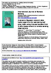
Figure 5: Example analysis of the first 5 s of Chopin's Nocturne. Op. 9 No. 1 in form of a piano-roll plots. From top to bot- tom: the ground truth (MIDI data), notes ...
2009 IEEE Workshop on Applications of Signal Processing to Audio and Acoustics
October 18-21, 2009, New Paltz, NY
NOTE DETECTION WITH DYNAMIC BAYESIAN NETWORKS AS A POSTANALYSIS STEP FOR NMF-BASED MULTIPLE PITCH ESTIMATION TECHNIQUES Stanisław A. Raczy´nski, Nobutaka Ono, Shigeki Sagayama The University of Tokyo Graduate School of Information Science and Technology 7–3–1, Hongo, Bunkyo-ku, Tokyo 113-8656 Japan e-mail: {raczynski,onono,sagayama}@hil.t.u-tokyo.ac.jp ABSTRACT In this paper we present a method for detecting note events in the note activity matrix obtained with Nonnegative Matrix Factorization, currently the most common method for multipitch analysis. Postprocessing of this matrix is usually neglected by other authors, who use a simple thresholding, often paired with additional heuristics. We propose a theoretically-grounded probabilistic model and obtain very promising results due to the fact that it was able to capture basic musicological information. The biggest advantage of our approach is that it can be extended without much effort to include various information about musical signals, such as principles of tonality and rhythm. Index Terms— Dynamic Bayesian Networks, Nonnegative Matrix Factorization, multipitch analysis, note detection 1. INTRODUCTION Multiple pitch estimation is one of the central problems of the Music Information Retrieval (MIR) community. It serves as a backend for many tasks, such as automatic music transcription, chord detection, source separation etc. Its goal is to determine what are the frequencies of different pitched signals mixed together at a given time in the input musical signal. Survey of the methods used for multipitch estimation in the algorithms submitted to the MIREX 2008 competition [1] shows that the most popular technique is the Nonnegative Matrix Factorization (NMF) and its various extensions – more than half of the entries was based on it. However, NMF does not directly yield information about note onsets, offsets and pitches, but provides a matrix of estimated note amplitudes sometimes referred to as the note activity matrix.1 The same survey also shows that the note detection in the note activity matrix is performed with a simple thresholding, often paired with a set of heuristic rules. In this paper we present a more theoretically-grounded probabilistic framework for detecting notes in this matrix. 1.1. Nonnegative Matrix Factorization NMF [2], also called Nonnegative Matrix Approximation (NNMA) [3], is a method for decomposing a nonnegative (having only nonnegative elements) matrix X (later referred to as the 1 This might seem like an oversimplification, as the matrix obtained through NMF might not correspond to the note amplitudes, depending on the basis matrix used and various other factors. Further processing might be required to obtain the note activities, nevertheless the note activity matrix is the final product of this stage of multipitch analysis.
data matrix) into a product of two, also nonnegative, matrices A and S: e X∼ (1) = AS = X.
In other words, this method approximates each column of the data matrix with a linear combination of basis vectors at (columns of A): X sn,t at , (2) xet = n
where n is the basis vector number and t is the time index. This method has become important for researchers in the Music Information Retrieval field, especially for multipitch analysis task (see [4, 5, 6, 7]). It is used to decompose a nonnegative power or amplitude spectrogram of the analyzed musical signal into a linear combination of spectra of individual notes. The note activity matrix is assumed to contain the nonnegative amplitudes of individual notes, while the basis matrix A (also nonnegative) – spectra of these notes. 1.2. Graphical modeling
Graphical probabilistic models have been gaining popularity very fast in the last years. One of the biggest strengths of these models is the existence of ready-to-use inference tools that only require the user to specify the network structure (conditional dependencies) and the conditional probability distributions. A special kind of graphical models, Dynamic Bayesian Networks (DBNs), is of particular interest to the signal processing community. One of the simplest DBNs is the Hidden Markov Model (HMM), a twolayered model, virtually omnipresent in the community for nearly 30 years, without which speech recognition would be impossible. Even though HMM is sometimes used in MIR tasks, DBNs are still not widely known and there is only little research that uses them (of particular relevance to multipitch analysis is a different DBN-based approach presented by Cemgil [8] and an HMM-based approach presented by Emiya et al. [9]). 2. NOTE ACTIVITY ANALYSIS FRAMEWORK To deal with the task of analyzing the note activity matrix, we have designed a three-layer DBN, structure of which is presented in Fig. 1. The bottom layer of nodes Yt is the observed note activity and its first difference. Above it is the note combination layer Nt and, at the top, the transition layer Ct . The note combination variable Nt contains a set of piano keys being held at a particular moment in time, while the transition variable Ct is a simple binary
October 18-21, 2009, New Paltz, NY
0.2
0.02
(b) Thresholding as a DBN
0.0
0.00
(a) The proposed DBN
0.4
0.04
0.6
0.8
0.06
2009 IEEE Workshop on Applications of Signal Processing to Audio and Acoustics
0 0.14
Figure 1: The structure of dynamic Bayesian networks used in this paper.
0.34
0.54
0.74
0.94
0 0.14
PL (L)P (K|L) Q PL (L)P (K0 ) L l=1 PK (Kl−1 − Kl−1 )
0.04 0.00 −0.6
−0.2
0.2
0.6
1
−1
Difference of note activity
−0.6
−0.2
0.2
0.6
1
Difference of note activity
P∆s (∆si,t |i ∈ / Nt ∧ i ∈ / Nt−1 ) P∆s (∆si,t |i ∈ Nt ∧ i ∈ / Nt−1 ) 0.4
(7)
0.3 0.2
The note combination transition probability is given by: δNt ,Nt−1 if Ct = 0 , P (Nt |Ct , Nt−1 ) = PN (Nt,1 , Nt−1,1 )P (L, K) if Ct = 1 (8) where PN (Nt,1 , Nt−1,1 ) is a transition probability of the highest note (it is usual that the main melody takes place in the highest notes, as discussed by Uitdenbogerd [10]). The note combination probability is given by a first-order homogeneous Markov chain of length L. Its state is a piano key number. The transition matrix is a strictly lower triangle matrix, so the generated note sequence can only progress towards lower frequencies. = =
0.2 −1
0.1
=0 =1 . =0 =1
0.0
= 0 ∧ Ct−1 = 0 ∧ Ct−1 = 1 ∧ Ct−1 = 1 ∧ Ct−1
0.30
if Ct if Ct if Ct if Ct
0.20
8 a > < 1 1 − a1 P (Ct |Ct−1 ) = > a2 : 1 − a2
0.0
Ps (si,t |Nt )P∆s (∆si,t |Nt , Nt−1 ) (6)
i=1
P (L, K)
0.08
0.6
(5)
0.10
88 Y
Ps (si,t |Nt )
i=1
0.00
P (Yt |Nt , Nt−1 ) =
(4)
0.94
Figure 2: Distribution of the measured note activity depending on if the note was present or not.
0.4
P (Y0 |N0 ) =
88 Y
0.74
Ps (si,t |i ∈ / Nt )
0.8
P (N0 |C0 ) = P (L, K),
0.54
Note activity
Ps (si,t |i ∈ Nt ) yes-no value that determines whether the transition from one note combination to another is allowed or not. The conditional probabilities of the network are defined as follows: 1 if C0 = 0 , (3) P (C0 ) = 0 if C0 = 1
0.34
Note activity
−1
−0.6
−0.2
0.2
0.6
1
−1
Difference of note activity
−0.6
−0.2
0.2
0.6
1
Difference of note activity
P∆s (∆si,t |i ∈ / Nt ∧ i ∈ Nt−1 )P∆s (∆si,t |i ∈ Nt ∧ i ∈ Nt−1 ) Figure 3: Distribution of the measured note activity difference depending on the change of state of the corresponding note.
(9)
2.1. Model parameters All models parameters (conditional probability distributions) were trained on a dataset of synchronized MIDI and audio files containing live piano renditions of most of Fryderyk Chopin’s pieces recorded on a MIDI piano [11]. Estimated note combination probabilities PK , PK0 , PN and PL were trained on the MIDI files and are depicted in Fig. 4. The output probabilities Ps and P∆s were trained on MIDI and audio files and are depicted in Fig. 2 and 3. Temporal parameters a1 and a2 were estimated to be equal to 0.814 and 0.644, respectively. 2.2. Note combination selection The number of all possible note combinations is enormous. For example, if all combinations of piano keys are allowed, we get
over 3.1 × 1026 different states of the Nt variable, and it is obviously computationally impossible to check all these combinations. In our approach, to deal with this problem, only M note combinations are selected for each time frame to be used in the analysis, together with the note combination selected in the previous 2 time frames. The selection is based on the fitness measure calculated for each note combination candidate as:
F (Nt ) =
P L
st,i , i st,i
i∈Nt
P
(10)
where L is the length of evaluated note combination Nt . The list of candidates is first created as a list of all possible combinations of K biggest note activities, resulting in 2K note combination candidates being evaluated at each time frame.
2009 IEEE Workshop on Applications of Signal Processing to Audio and Acoustics
October 18-21, 2009, New Paltz, NY
CT = E I [NT ],
To additionally increase the accuracy of the proposed method, a pre-thresholding was introduced to discourage the algorithm from detecting spurious notes and increase the precision. This was achieved by reducing all output probabilities Ps corresponding to values smaller than the threshold to zeros.
0.00
0.00
0
2
Piano key number
4
6
8 10
13
16
Note combination length
(a) PK0 (K0 )
(b) PL (L)
3. EXPERIMENTAL RESULTS
0.15
0.12
(25)
2.4. Pre-thresholding
1 9 19 31 43 55 67 79
0.00
0.00
0.05
0.04
0.10
0.08
(24)
BtI [Nt , Ct+1 ].
Ct =
0.10
0.02
0.20
0.04
Nt =
(23)
DtI [Ct+1 , Nt+1 ],
1 9 19 31 43 55 67 79
−62 −42 −22 −4 9 22 37 52
Transition interval
Transition interval
(c) PK (Kl−1 − Kl−1 )
(d) PN (Nt,0 , Nt−1,0 )
Figure 4: Note combination probabilities: (a) highest note distribution, (b) combination length distribution, (c) note transition probability (note that a distinct repeating octave-long pattern is visible, with peaks at the minor and major thirds, perfect fifth and an octave), (d) highest note transition distribution. 2.3. Inference The inference is performed by the Frontier Algorithm [12], modified to find the optimal path through hidden states. At initial time frame, a single array is calculated: D0 [C0 , N0 ] = P (C0 )P (N0 |C0 )P (Y0 |N0 ),
(11)
and the following arrays are calculated iteratively for each time t = 2, 3, ..., T of the analyzed data: At [Ct−1 , Nt−1 , Ct ] = Dt−1 P (Ct |Ct−1 ),
(12)
Bt [Nt−1 , Ct ] = max At ,
(13)
BIt [Nt−1 , Ct ]
Ct−1
= arg max At , Ct−1
(14)
Ct [Nt−1 , Ct , Nt ] = Bt P (Nt |Ct , Nt−1 )P (Yt |Nt , Nt−1 ), (15) Dt [Ct , Nt ] = max Ct , (16) DIt [Ct , Nt ]
Nt−1
= arg max Ct . Nt−1
The algorithm finishes by calculating: E[NT ] = max DT , CT
(17)
(19)
F = max E,
(20)
I
NT
F = arg max E. NT
(21)
The BI and DI arrays are stored for each time frame and used for backtracing in the last step of the algorithm: NT = F I ,
Method Threshold Song “Wiosna” Nocturne op. 9 no. 2 Bolero op. 19 Nocturne op. 32 no. 1 Etude op. 10 no. 3 Nocturne op. 9 no. 1 Ballade op. 38 no. 2 Fantasie-impromptu op. 66 Mazurka “Notre Temps” Etude “Revolutionary” average
Thresholding 0.16 best 95.5% 97.2% 82.5% 84.2% 91.4% 94.3% 71.7% 81.7% 50.3% 68.3% 88.1% 84.4% 79.9% 84.0% 73.6% 80.1% 85.1%
Proposed DBN 0.12 best 98.1% 99.1% 88.8% 88.8% 87.3% 89.2% 83.1% 94.6% 59.5% 80.0% 88.2% 82.7% 77.3% 83.1% 73.7% 82.2% 90.3%
Table 1: F-measures obtained for thresholding and the proposed Bayesian network. One set of results corresponds to using a fixed, globally optimized threshold and the other to the best obtainable value.
(18)
EI [NT ] = arg max DT , CT
Figure 5: Example analysis of the first 5 s of Chopin’s Nocturne Op. 9 No. 1 in form of a piano-roll plots. From top to bottom: the ground truth (MIDI data), notes detected using the proposed framework (pre-thresholding at 0.14), and notes detected by thresholding with an optimal threshold of 0.26. F-measure is 100% and 89% accordingly. Note that note duration is generally better estimated with the DBN.
(22)
To evaluate our approach, we have created an experimental environment similar to the one used in the MIREX competition’s piano transcription sub-task. Accuracy of note detection was evaluated with the F-measure. The Chopin dataset, consisting of 216 synchronized MIDI and audio files, was divided into the training subset and the validation subset and 20-fold validation was used. In the experiments, K was set to 6 (effectively limiting the polyphony to 6 concurrent pitches) and M = 100 note combination was selected at each frame. Following MIREX evaluation
0.6 0.2
0.4
F−measure
0.6 0.4 0.0
0.0
0.2
F−measure
0.8
0.8
1.0
2009 IEEE Workshop on Applications of Signal Processing to Audio and Acoustics
0.0
0.1
0.2
0.3
0.0
0.4
0.1
0.2
0.3
0.4
Threshold
Threshold
Etude Op. 10 No. 3 0.8
notes. The obtained results are very promising and generally better than thresholding. Not only we have observed an increase in the average F-measure, but also a better estimation of the note offset times (compare Fig. 5). Furthermore, the proposed model was much more robust to parameter changing than the simple thresholding (compare Fig. 6). The biggest strength of the proposed approach is its flexibility: the Bayesian network can be extended extremally easy by adding additional nodes or using more complex conditional probability distribution. It is our current goal to extend it to incorporate more musicological information, such as tonal progression and to achieve more precise note length modeling.
0.6
5. REFERENCES
0.2
0.4
F−measure
0.6 0.4 0.2
0.0
0.0
F−measure
0.8
Song Op. 74 “Wiosna”
October 18-21, 2009, New Paltz, NY
0.0
0.1
0.2
0.3
0.4
Threshold
Nocturne Op. 9 No. 2
0.0
0.1
0.2
0.3
0.4
Threshold
Bolero Op. 19
Figure 6: Results obtained for different threshold value. Black solid line shows results obtained for the proposed method, while the dark gray dashed line for simple thresholding.
method, notes were assumed correctly detected if the estimated onset time was within 50 ms of the onset time recorded in the MIDI data. The I-divergence NMF was used with 3 different fixed basis matrices and the resulting 3 note activity matrices were geometrically averaged together (to emphasize values shared between them and decrease the amount of spurious note activity) and used as input data. All 3 basis matrices contained 88 basis vectors corresponding to keys on a standard piano keyboard (notes from 21 to 108 on the MIDI scale). The first basis was filled with harmonically structured vectors shaped with an envelope exponentially decaying -6 dB per octave. The second and third basis matrices were trained on the training subset of the Chopin dataset with MIDI data serving as fixed note activity matrix, one with a harmonic constrain[13], the other without. Time precision was set to 20 ms. Results obtained with the proposed DBN were compared to results obtained with the de facto standard for note activity matrix analysis – thresholding, that can be emulated by the proposed DBN by adjusting the probability distributions in a manner that reduces the network to a DBN depicted in Fig. 1 (b). Therefore our expectation was to outperform thresholding due to the fact that much more musical knowledge is encoded in the proposed network. For each piece of music, the first 30 s were analyzed. Summary of the results can be found in Table 1. The resulting F-measures as a function of threshold for first 4 of the files are depicted in Fig. 6. Additionally, analysis results of the first 5 seconds of one of Chopin’s nocturnes are presented in Fig. 5. 4. CONCLUSION AND FUTURE WORK In this paper we have presented a probabilistic framework for note detection that extends thresholding by incorporating basic musical knowledge, such as e.g. distribution of common intervals between notes that make up a chord or distribution of the number of these
[1] “MIREX 2008 multiple fundamental frequency estimation and tracking results,” May 2009. [Online]. Available: http://www.music-ir.org/mirex/2008/ index.php/Multiple Fundamental Frequency Estimation % 26 Tracking Results [2] D. Lee and H. Seung, “Algorithms for Non-negative Matrix Factorization,” Advances in Neural Information Processing Systems, pp. 556–562, 2001. [3] I. Dhillon and S. Sra, “Generalized Nonnegative Matrix Approximations with Bregman divergences,” Advances in Neural Information Processing Systems, vol. 18, p. 283, 2006. [4] P. Smaragdis and J. Brown, “Non-negative Matrix Factorization for polyphonic music transcription,” in Proc. of IEEE WASPAA, 2003, pp. 177–180. [5] S. Abdallah and M. Plumbley, “Unsupervised analysis of polyphonic music by sparse coding,” IEEE Trans. Neural Netw., vol. 17, no. 1, pp. 179–196, 2006. [6] M. Schmidt and M. Mørup, “Sparse Non-negative Matrix Factor 2-D Deconvolution for automatic transcription of polyphonic music,” in Proc. 6th International Symposium on Independent Component Analysis and Blind Signal Separation, 2006. [7] E. Vincent, N. Bertin, and R. Badeau, “Harmonic and inharmonic nonnegative matrix factorization for polyphonic pitch transcription,” in Proc. of IEEE ICASP, 2008, pp. 109–112. [8] A. Cemgil, B. Kappen, and D. Barber, “Generative model based polyphonic music transcription,” in Proc. of IEEE WASPAA, 2003. [9] V. Emiya, R. Badeau, and B. David, “Automatic transcription of piano music based on HMM tracking of jointly-estimated pitches,” in Proc. of EUSIPCO. [10] A. Uitdenbogerd and J. Zobel, “Melodic matching techniques for large music databases,” in Proc. of the seventh ACM international conference on Multimedia (Part 1). ACM New York, NY, USA, 1999, pp. 57–66. [11] “The ultimate Chopin MIDI collection,” May 2009. [Online]. Available: http://www.geocities.com/Vienna/2217/midi.htm [12] K. Murphy, “Dynamic Bayesian networks: representation, inference and learning,” Ph.D. dissertation, University of California, 2002. [13] S. Raczy´nski, N. Ono, and S. Sagayama, “Multipitch analysis with Harmonic Nonnegative Matrix Approximation,” in Proc. of the 8th ISMIR, 2007.