prediction accuracy, 88.85%, is obtained by bigram dynamic ... malsâ, while a stricter definition in an academic presentation .... Unigram DB classification.
DYNAMIC BAYESIAN SOCIO-SITUATIONAL SETTING CLASSIFICATION Yangyang Shi, Pascal Wiggers, Catholijn M. Jonker Delft University of Technology Department of Mediamatics Mekelweg 4, 2628 CD Delft, NL ABSTRACT We propose a dynamic Bayesian classifier for the sociosituational setting of a conversation. Knowledge of the sociosituational setting can be used to search for content recorded in a particular setting or to select context-dependent models in speech recognition. The dynamic Bayesian classifier has the advantage – compared to static classifiers such a naive Bayes and support vector machines – that it can continuously update the classification during a conversation. We experimented with several models that use lexical and part-of-speech information. Our results show that the prediction accuracy of the dynamic Bayesian classifier using the first 25% of a conversation is almost 98% of the final prediction accuracy, which is calculated on the entire conversation. The best final prediction accuracy, 88.85%, is obtained by bigram dynamic Bayesian classification using words and part-of-speech tags. Index Terms— Dynamic Bayesian networks, conversation classification, socio-situational setting 1. INTRODUCTION “You shall know a word by the company it keeps” [1]. We also shall know a conversation by the situation in which it is used. This situation is characterized by several aspects, such as conversation goals, the number of speakers and listeners, the relation among the speakers and listeners and the conversation medium. In different socio-situational settings, people may demonstrate differences in their pronunciation, word choice and grammar use [2]. For example, one might explain the definition of “Artificial Intelligence ” to a friend in a vivid as “a system designed to mimic the behaviors of humans or animals”, while a stricter definition in an academic presentation might be “The study and design of intelligent systems . . . ”. The socio-situational setting of a conversation – whether it is a spontaneous conversation by phone or face to face, a lecture in a classroom or a political debate – is independent of the topic of a conversation and related to, but different from a conversation’s genre. Topics relate to conversation content. Different types of conversations can relate to the same topics.
978-1-4673-0046-9/12/$26.00 ©2012 IEEE
5081
For example, one might want to search a lecture on “Western civilization”, rather than a political debate which refers to “Western civilization”. A genre has a set of stylistic and rhetoric characteristics and some content related aspects. For example, a text or conversation may be classified as science fiction or as a reportage. In contrast, the socio-situational setting, as we use it here, classifies a conversation into categories such as spontaneous face-to-face conversations, lectures or debates. Traditional conversation classification methods are based on text classification. The text of the entire conversation is used to find the socio-situational setting. Intuitively, however only a small amount of text may be sufficient to provide a reasonable guess of the socio-situational setting. For example, a conversation beginning with “In this class, we will . . . ” is likely to be a lecture, and a conversation starting with “Hello, this is Mike speaking.” probably is a spontaneous conversation by phone. Therefore, dynamic classification methods update the class prediction during the conversation. Such dynamic classification methods can be used for example to select a situation-specific language model on the fly [3, 4]. In this paper we present an approach to dynamic classification of the socio-situational setting. In particular we studied if it is sufficient to use only the initial part of a conversation to make an accurate prediction of the socio-situational setting. The paper is organized as follows. The next section briefly discusses related work. In section 3, we introduce dynamic Bayesian networks and present our dynamic Bayesian classifiers. The experiments we conducted are described in section 4. Finally, based on the results, conclusions are drawn. 2. RELATED WORK Socio-situational setting classification is related to classic genre classification. As defined by Kessler [5], the genre is the way a text is created, the way it is distributed, the register of language it uses and the kind of audience it is addressed to, such as an Editorial, a Reportage or a Research article. In language processing, parsing accuracy, part-of-speech (POS) tagging accuracy and word-sense disambiguation can be enhanced by taking genre information into account.
ICASSP 2012
Classification of the genre or the social situation is typically done based on all words in a segment of text [6, 7]. Classifiers used include decision trees, neural networks, support vector machines and K-nearest neighbors classifiers [8]. Naive Bayesian (NB) classifiers described by [9], are seen as the most important probabilistic classifiers in document classification. A chain augmented naive Bayesian (CAN) classifier [10] can be viewed as a combination of a NB and a ngram language model. It determines the category by maximizing the likelihood of a sequence of word given class label. However, none of these works tried to dynamic update prediction during a conversation.
posterior probability P (C = c|D = d): {P (C = ci |D = d)}, c∗ = arg max i c ∈C
= arg max { i c ∈C
P (C = ci ) × P (D = d|C = ci ) }. P (D = d)
(2) (3)
The DB method differs from this general approach in that it updates the classification for every word that is observed: c∗ = arg max {P (Ct = ci |D1:t = d1:t )}, i c ∈C
(4)
where Ct is the class variable at time step t and d 1:t is the observed document information from time step 1 to t. Let αt (i) = P (Ct = ci |D1:t = d1:t ).
(5)
Using the forward algorithm for DBNs [12], α t can be calculated in an iterative way. Take the DB classification model in Fig.1 as an example,
3. DYNAMIC BAYESIAN DOCUMENT CLASSIFICATION 3.1. Features Three simple features are used in dynamic Bayesian sociosituational setting classification: words, POS-tags and sentence length. As are discussed in [7, 11], the distribution of these features varies in different socio-situational settings. For example, in news report, more nouns and articles are used than in spontaneous conversations, while in in the later, more adjectives are used on average than in formal conversations, such as political debates/discussions and sermons. The sentences in spontaneous speech are considerably shorter than in formal conversations.
α1 (i) = αt (i) =
P (C1 = ci ) × P (D1 = d1 |C1 = ci ) , (6) P (D1 = d1 ) � i j j∈[1,n] (P (Ct = c |Ct−1 = c ) × αt−1 (j)) P (Dt = dt |D1:t−1 = d1:t−1 )
(7)
i
× P (Dt = dt |Ct = c ). At every time step, the class label can be updated by selecting the class that maximizes the posterior probability: c∗ = arg max αt (i). i c ∈C
(8)
Actually both the NB and CAN classification methods are
3.2. Dynamic Bayesian networks Dynamic Bayesian networks (DBNs) [12] extend Bayesian networks. They can model probability distributions of semiinfinite sequences of variables that evolve over time. A DBN can be represented by a prior model P (X 1 ) and a two slice temporal Bayesian network which defines the dependence between a particular step and previous step: P (Xt |Xt−1 ) =
N �
P (Xti |P a(Xti ))
(1)
i=1
where Xt is the set of random variables at time t and X ti is the ith variable in time step t. P a(X ti ) are the parents of X ti . 3.3. Dynamic Bayesian document classifier We classify conversations based on their lexical transcripts. This can be seen as document classification, which maps a document d to one of a set of predefined classes C = {c1 , c2 , ..., cn }. DB classification is a conditional probabilistic classification method. Probabilistic classification makes a prediction by seeking a category which maximizes the
5082
Fig. 1. Examples of Bayesian classifiers, the left one is NB, the middel is DBN classifier, the right one is trigram DBN classifier using word and POS particular dynamic Bayesian classification methods under the condition that P (Ct = ci |Ct−1 = ci ) = 1. When the whole document is observed, and if we assume that there is no dependency between the d t s, it is a NB classification method. If there is a Markov chain dependency between d t−1 and dt , it comes down to the CAN classification method. 4. EXPERIMENT We experimented with nine different dynamic Bayesian classifiers for socio-situational setting classification. These models differ in the features used and in the relations between the features modelled.
4.1. Data The models are trained and tested on the transcriptions of the Corpus Spoken Dutch (Corpus Gesproken Nederlands, CGN ) [13]. This corpus consists of transcribed audio recordings of Dutch, divided into 14 components that correspond to socio-situational settings such as spontaneous face to face conversations, simulated business negotiations, lectures and read speech. The corpus contains almost 9 million words. In this experiment, a vocabulary of 44368 words was created, which contains all words that occur more than once in the training data. The words not in the vocabulary were treated as an out-of-vocabulary token. 80% of CGN is used for training, 10% for development and the remaining 10% for evaluation.
Take the trigram DB classifier that uses only words as an example, at time step t, wt depends on c t , wt−1 and wt−2 . The conditional probability is represented as an interpolation: Pint (wt |wt−1 , wt−2 , ct ) = λ1 P (wt |wt−1 , wt−2 , ct ) + λ2 P (wt |wt−1 , ct ) + λ3 P (wt |ct ) + λ4 P (wt ).
4.2.5. Trigram DB classification using combination of words and POS In this model (Fig. 1), the POS-tags are conditioned on the previous two POS-tags using equation (13). w t depends on previous two words w t−1 , wt−2 , as well as on the current post and on the class label c t .
4.2.1. Unigram DB classification
Pint (wt |wt−1 , wt−2 , post , ct ) = λ1 P (wt ) + λ2 P (wt |ct ) + λ3 P (wt |wt−1 , ct ) + λ4 P (wt |post )
The unigram DB classification equals naive bayesian classification. The interpolated conditional probability of words the in unigram DB classification method is,
+ λ7 P (wt |wt−1 , wt−2 , post ) + λ8 P (wt |wt−1 , wt−2 , post , ct ).
4.2. Models
Pint (wt |ct ) = λ1 P (wt ) + λ2 P (wt |ct ).
(9)
In case of using the combination of words and POS-tags, the interpolated probability is, Pint (wt |post , ct ) = λ1 P (wt ) + λ2 P (wt |ct ) + λ3 P (wt |post ) + λ4 P (wt |, post , ct ).
(10)
4.2.2. Bigram DB classification only using word or POS These two models are under the assumption of a 1-order Markov chain. The features at a particular time step t only depend on the features at t − 1 and the current hidden variable ct . The interpolated conditional probability is: Pint (wt |wt−1 , ct ) = λ1 P (wt |wt−1 , ct ) + λ2 P (wt |wt−1 ) + λ3 P (wt ).
(11)
4.2.3. Bigram DB classification using combination of words and POS For this model each POS-tag is conditioned on the previous POS -tag using equation (10). The interpolated conditional probability of a word in this case is: Pint (wt |wt−1 , post , ct ) = λ1 P (wt ) + λ2 P (wt |ct ) + λ3 P (wt |wt−1 , ct ) + λ4 P (wt |post )
(12)
+ λ5 P (wt |wt−1 , post ) + λ6 P (wt |wt−1 , post , ct ). 4.2.4. Trigram DB classification only using words or POS The 2nd order Markov chain is applied in these two models. Words or POS-tags are used as features of a conversation.
5083
(13)
+ λ5 P (wt |wt−1 , wt−2 , ct ) + λ6 P (wt |wt−1 , post )
(14)
In the equations (9),(10),(11),(12),(13) and (14), all inter� polated parameters λ i ∈ [0, 1] and λi = 1. These parameters are trained on the held-out development set. 4.3. Results In terms of overall performance, the DB classifier using POStag and word bigrams, which achieves a prediction accuracy of 88.85%, performs best among the 9 classifiers. Actually, unigram DB classifier using 100% information performs like traditional naive Bayesian classifier. Fig. 2 shows the prediction accuracy of the 9 classifiers as a function of the percentage of test data observed. The exact prediction accuracies of 9 classifiers with 25, 50 and 100 percent data are listed in Table 1. As Fig. 2 shows, the prediction accuracy increases rapidly for the first 20% of the data. After that the trend becomes flat. The DB classifiers using only words are more stable and precise than systems that use only POS-tags. Based on 1% of the information, both trigram and bigram DB classifiers using words can get over 70% prediction accuracy, while systems that use only POS-tags achieve less than 65% accuracy. We also tested classifiers that included the sentence length as a feature, but none of these models showed a significant improvement over the corresponding model without the sentence length variable. 5. CONCLUSION Socio-situational setting classification of conversations was introduced in this paper. A DB classification method was proposed, which provides a dynamic continuous strategy for conversation classification. We experimented with 9 different DB socio-situational setting classifiers. The bigram DB
trigram only word
trigram only pos 1
1
0.9
0.9
0.9
0.8
0.8
0.8
0.7
0.7
0.7
0.6
0.6
20
40
60
80
100
r(25)=0.97112,y(100)=0.8697
20
40
60
80
100
r(25)=0.94843,y(100)=0.85243
bigram only word
0.6
bigram only pos 1
0.9
0.9
0.9
0.8
0.8
0.8
0.7
0.7
0.7
40
60
80
100
0.6
20
40
60
80
100
0.6
40
60
80
100
20
40
60
80
r(25)=0.96113,y(100)=0.88854
unigram only word
unigram only pos
unigram word and pos
1
1
0.9
0.9
0.9
0.8
0.8
0.8
0.7
0.7
0.7
0.6
0.6
20
40
60
80
100
20
40
60
80
100
r(25)=0.93083,y(100)=0.79435
0.6
POS
word, POS word POS
word, POS word
100
r(25)=0.95817,y(100)=0.82575
r(25)=0.94526,y(100)=0.86028
Trigram
Bigram
r(25)=0.9556,y(100)=0.88383 1
information word
20
bigram word and pos
1
20
models
r(25)=0.97861,y(100)=0.88069
1
0.6
Table 1. The prediction accuracy of 9 classifiers
trigram word and pos
1
Unigram
POS
word, POS
20
40
60
80
cation of text,” in IEEE International Conference on Acoustics, Speech and Signal Processing, 2009, pp. 4781 –4784.
100
r(25)=0.96125,y(100)=0.85086
Fig. 2. Prediction accuracy trend over percent of each conversation, x,y axis represent the percentage of a conversation and prediction accuracy, respectively. y(100) represent prediction accuracy using 100% information, r(25) = y(25)/y(100)
[7] Yangyang Shi, Pascal Wiggers, and Catholijn M. Jonker, “Socio-situational setting classification based on language use,” in IEEE workshop on automatic speech recognition and understanding, 2011. [8] Fabrizio Sebastiani, “Machine learning in automated text categorization,” ACM Comput. Surv., vol. 34, pp. 1–47, March 2002.
socio-situational setting classification method obtained the best result, 88.85% final prediction accuracy. We found that when using only the first 25% of a conversation the classification equals the result found when using information from the whole conversation in 94% of the cases.
[9] Pat Langley, Wayne Iba, and Kevin Thompson, “An analysis of bayesian classifiers,” in proceedings of the tenth national conference on artificial intelligence. 1992, pp. 223–228, MIT Press.
6. REFERENCES [1] John R. Firth, “A synopsis of linguistic theory, 19301955,” Studies in Linguistic Analysis, pp. 1–32, 1957. [2] W. Labov, Sociolinguistic patterns, University of Pennsylvania Press, 1972. [3] Yangyang Shi, Pascal Wiggers, and Catholijn M. Jonker, “Language modelling with dynamic bayesian networks using conversation types and part of speech information,” in The 22nd Benelux Conference on Artificial Intelligence, 2010. [4] Yangyang Shi, Pascal Wiggers, and Catholijn M. Jonker, “Combining topic specific language models,” in Text, Speech and Dialogue (TSD), 2011. [5] Brett Kessler, Geoffrey Numberg, and Hinrich Sch¨utze, “Automatic detection of text genre,” in Proceedings of the eighth conference on European chapter of the Association for Computational Linguistics, 1997, pp. 32–38.
prediction accuracy 25%data 50%data 100%data 84.46% 84.93% 86.97% 80.85% 83.05% 85.24% 86.19% 86.19% 88.07% 84.46% 85.56% 88.38% 79.12% 81.00% 82.57% 85.40% 86.81% 88.85% 81.32% 84.14% 86.03% 73.94% 76.92% 79.43% 81.79% 83.99% 85.09%
[10] Fuchun Peng and Dale Schuurmans, “Combining naive bayes and n-gram language models for text classification,” in 25th European Conference on Information Retrieval Research, 2003, pp. 335–350. [11] Pascal Wiggers and Leon J. M. Rothkrantz, “Exploratory analysis of word use and sentence length in the Spoken Dutch Corpus,” in Text, Speech and Dialogue, 2007. [12] Kevin Murphy, Dynamic Bayesian Networks: Representation, Inference and Learning, Ph.D. thesis, University of California, Berkeley, 2002. [13] Nelleke Oostdijk, Wim Goedertier, Frank Van Eynde, Louis Boves, Jean pierre Martens, Michael Moortgat, and Harald Baayen, “Experiences from the spoken dutch corpus project,” in Araujo (eds), Proceedings of the Third International Conference on Language Resources and Evaluation, 2002, pp. 340–347.
[6] S. Feldman, M.A. Marin, M. Ostendorf, and M.R. Gupta, “Part-of-speech histograms for genre classifi-
5084