Dynamic Behavior of Current Controllers for Selective Harmonic Compensation in Three-phase Active Power Filters Fernando Briz, David Díaz-Reigosa, Michael W. Degner†, Pablo García, Juan Manuel Guerrero University of Oviedo, Dept. of Elec., Computer & Systems Engineering Gijón, 33204, Spain T: 34 985-182289, E:
[email protected] Abstract –. Current regulators are a critical part of active power filters (APF's). Design of current regulators capable of compensating high frequency harmonics created by non-linear loads is a challenging task. Selective harmonic current compensation using harmonic regulators is a viable method to achieve this goal. However, their design and tuning is not an easy task. The performance –and even the stability- of harmonic current regulators strongly depends on implementation issues, with the tuning of the controller gains being critical. Furthermore, the presence of multiple current regulators working in parallel can create unwanted couplings with the fundamental current regulator, which can result in a deterioration of APF current control, i.e., oscillations and settling times larger than expected.. This paper addresses the design and tuning of selective harmonic compensators, with a focus on their stability analysis and transient behavior.
†HEV and FCEV Research Dept, Research and Advanced Engineering, Ford Motor Company 2101 Village Road, MD 1170, Dearborn, MI 48121-2053, T: 313-322-6499, E:
[email protected] that they can totally cancel the harmonics included in their design, including the ability to dynamically select the harmonics to compensate when the magnitude of the harmonic currents surpass the APF's capability. Concerns for the implementation of harmonic current regulators include their computational requirements, tuning, and circuit configuration. While first one is becoming less important thanks to fast and relatively cheap digital signal processors, selection of the gains for the controllers, as well as circuit configuration options, to guarantee stable operation and adequate dynamic performance is a challenge. Power grid
I. INTRODUCTION Shunt active power filters (APF) are power electronic devices designed for the compensation of harmonic current from nonlinear loads, which also have the capability of compensating reactive power and unbalanced loads, see Fig. 1 [1-12]. The current controller is a critical component of these APF's with the choice available of regulating either the line currents [1], Fig. 1 and the block diagram shown in Fig. 2a, or the active filter currents, the block diagram shown in Fig. 2b [1,5,8]. The first option has the advantage that only the line current needs to be measured. The second option requires measurement of both the APF currents and the line currents, which are needed for determining the harmonics that need to be decoupled, but has the advantage of providing over-current protection for the APF. From a dynamic point of view both solutions are similar and the first one will be used in this paper [1]. A number of current control strategies for APF have been proposed, including hysteresis, linear (PI), sliding and deadbeat controllers [6,7]. These methods normally have significant limitations eliminating harmonics injected by nonlinear loads. Selective harmonic compensation was developed to address these concerns and is a control strategy in which several (normally linear) harmonic current regulators work in parallel, each canceling a specific harmonic injected by the load [6-12]. An appealing property of these methods is Τhis work was supported in part by the Research, Technological Development and Innovation Programs of the Spanish Ministry of Science and Innovation −ERDF under grant MICINN-10-ENE2010-14941 and the Ministry of Science and Innovation under grant MICINN-10-CSD2009-00046.
il
vl
a,b,c d,q
iload Non-linear loads iF
a,b,c d,q
s
Lf, Rf
is
vlqd
lqd
vF e−jθe e−jθe e e vld ilqd e e e* − * − * * ild ilqd Vdc current vFqd reg. − Vdc e ilq* PWM Vdc inverter Fig. 1.- Block diagram of a parallel APF, including line current and DC bus voltage control. velqd
a) e* ilqd −
GFCR
* veFqd
+
e PWM vFqd inverter GLPF (optional)
b)
e* iFqd −
GFCR +
* veFqd
e PWM vFqd inverter
e iload qd iFqd + ie lqd − e
− GF
velqd − GF
e iload qd e iFqd + ie lqd −
GLPF (optional) Harmonic detection
Fig. 2.- Schematic representation of the APF qd current control shown in a synchronous reference frame (outer dc-link voltage control not shown). a) line current is regulated, b) active filter current is regulated. GFCR stands for fundamental current regulator transfer function, GF for the inductive filter transfer function and GLPF for the (optional) low-pass filter in the current feed back.
500 0 -500
a) vuv, vvw, vwu, (V) b) iload u, iload v, iload w (A) c) Line voltage harmonics (pu)
500
0.52
0
0.54
-500 0
0.25
0.5
0.75 4 0 -4
4
0.52
0 -4 0.040
1
0.25
0.5
0.75
1.25
0.54
1
1.25
h=7, −11, 13, −17 0
1
0.25
0.5
d)
h=−5
Load 0.5 currents harmonics 0 (pu)
h=7
0.75
1
h=1 h=−11, 13, −17
0.25
0.5
0.75
1
time (s)
Fig. 3.- Current drawn by an electric drive during an acceleration transient. The drive was connected to the line through a diode rectifier. a) line voltages, b) diode rectifier (load) phase currents, c) harmonic content of the line voltage, in pu of the fundamental component (h=1), d) harmonic content of the load current, in pu of the maximum value of the fundamental component: h=1
This paper analyzes the design, tuning and implementation of harmonic current regulators. Continuous models will be developed first for this analysis, since they make it easier to present the concepts involved. The effects due to a digital implementation of the harmonic current regulators will then be presented, with the goal of maintaining the stability and performance of the resulting discrete current regulators. II. PARALLEL ACTIVE POWER FILTER CONTROL An example block diagram of an APF is shown in Fig. 1. The line current references are generated from an outer dc-link voltage control loop and the supply line voltages. These current references are the ideal line currents, free of any high frequency harmonics demanded by the load and with the ability to provide any desired power factor, up to the limits of the APF. Fig. 2a shows the schematic representation of the APF current control in a reference frame synchronous with the line voltage vector. It can be noticed from Fig. 2a that the plant dynamics included in this model represent the dynamic characteristics of the APF output filter. An inductive filter, modeled as an RL load, is used for these purposes in Fig. 1 [3,5,7-11], with the corresponding transfer function being (1). It should be noted, however, that other options, like an LCL filter, can also be used with the appropriate changes in the plant model (1). e iFqd 1 GF = = (1) e e Lf (s+jωe)+Rf vFqd−vlqd
A.- Current harmonics due to non-linear loads The line voltages and load currents are disturbances to the system. In a synchronous reference frame, the fundamental line voltage becomes a dc quantity and is, therefore, easily compensated by a synchronous frame current regulator. On the other hand, some loads, e.g., diode rectifiers, create currents with a large content of high frequency harmonics. Compensation of the load currents is therefore a much more challenging task. The current harmonics created by non-linear loads typically have orders of h=−5, 7, −11, 13, … in the stationary reference frame, with h=1 corresponding to the fundamental frequency, ωe. These harmonics become h=±6, ±12, ±18 ... , when transformed to the synchronous reference frame [7,8]. Fig. 3 shows the experimentally measured currents drawn by an electric drive from the line during an acceleration transient, as well as the line voltage. Fig. 1c shows the variation over the time of the harmonics in the line voltage, while Fig. 1d shows the harmonics created by the load, both calculated using the Short-time Fourier Transform. It can be observed from the figure that the harmonics in the currents can change relatively quickly, reaching noticeably large values (relative to the fundamental current). The line voltage harmonics, on the other hand, show minimal change due to the transient currents created by the electric drive during its acceleration. The APF current regulator, therefore, needs to be able to cancel current harmonics that can be at frequencies relatively large compared to the fundamental frequency and has to provide good dynamic response, since these harmonics can change relatively fast. B.- Synchronous frame PI current regulators Synchronous frame PI current regulators have been widely used for the control of three-phase power converters [12]. The transfer function of a synchronous reference frame PI current regulator implemented in the synchronous reference frame is shown in (2). A pole-zero notation will be used throughout the paper, with the notation using the proportional Kp and integral Ki gain being indicated in (2). e∗ v (s + 1/Ti) Ki Kp qd GFCR = = Kp = Kp + ; Ki = (2) e s s Ti eqd To evaluate and compare the performance of different current regulators designs, it is useful to use the command tracking, i.e., output−to−reference, (3), and the disturbance rejection, i.e. output−to−disturbance, (4), transfer functions, shown in a synchronous reference frame e il_qd GFCR GF = (3) e∗ 1+GFCR GF GLPF i_ l qd e il_qd 1 = (4) e 1 + GFCR GF GLPF iload_qd
a) e i lqd(jω) e∗ i lqd(jω)
ve * GHCR_1
0.5
-42 -36 -30 -24 -18 -12 -6
e i lqd(jω) e load qd(jω)
0
6 12 18 24 30 36 42
1
0
a)
b) s iload qd (A)
2 0 -2 0 2
0.02 0.04 0.06 0.08 0.1 0.12 0.14 0.16 0.18 0.2
0 -2 0 2
c)
GHCR_2
s ilqd
0
(A)
-2 0
0.02 0.04 0.06 0.08 0.1 0.12 0.14 0.16 0.18 0.2
0.02 0.04 0.06 0.08 0.1 0.12 0.14 0.16 0.18 0.2 time (s)
Fig. 5.- Time response of an APF with a synchronous reference frame PI current regulator (simulated): a) line-current command, b) load current, consisting of harmonics h=±6, ±12, ±18, ±24 and ±30, c) actual line current. All the currents are shown in the stationary reference frame.
with GFCR standing for the fundamental current regulator transfer function in a synchronous reference frame (2), GF (1) being the APF inductive filter transfer function and GLPF being the transfer function of the low-pass filter in the current feedback, which can be optional depending on the current measurement strategy. A convenient way to analyze the performance of APF is through the use of frequency response function (FRF) analysis. Since the APF variables are modeled using complex vector quantities, which can rotate both forward and backwards, both positive as well as negative frequencies need to be considered for the transformation s=jω. Fig. 4-a and 4-b show the resulting FRF for (3) and (4), respectively. The current regulator was tuned to achieve pole/zero cancellation with a bandwidth of 400 Hz. The gains of the controller being Ti = Lf /Rf and Kp = 400 2 π Lf. It can be observed from Fig. 4-a that the FRF has a gain equal to one at 0 frequency, i.e., dc, which means they APF will have zero error in the steady-state. As for the disturbance rejection capability, current harmonics injected by non-linear
GHCR_n
* veFqd
+ +
* vehqd
+
GHCR
e
ilqd
b) e i *
−
* veqdh n
Kp
GFCR
+ e
a)
GFCR
+
qdh2
+
Kp
+
lqd
Fig. 4.- Frequency response function (FRF), shown in a synchronous reference frame, of the synchronous reference frame PI current regulator. The line frequency is ωe = 50 Hz, the harmonic order h being used for the frequency axis. The current regulator was tuned for a 400 Hz bandwidth (8·ωe) with no low-pass filter. a) Command tracking FRF (eq. (3)), and b) Disturbance rejection FRF (eq. (4)).
(A)
+
0.5
-42 -36 -30 -24 -18 -12 -6 0 6 12 18 24 30 36 42 harmonic order h
s* ilqd
qdh1
* veqdh
ve *
0
b)
i
e* ilqd −
1
ilqd
* veFqd
+ +
Kp
GHCR
* vehqd
c) Fig. 6.- a) Harmonic current regulator consisting of n parallel-connected regulators, b) current regulator consisting of a fundamental current regulator GFCR and a harmonic current regulator GHCR with the input to both current regulators being the current error, c) current regulator consisting of a fundamental current regulator and a harmonic current regulator with the input to the harmonic current regulator being the measured current.
loads will have typically orders of h=±6, ±12, ±18, ... , in the synchronous reference frame [7,8]. Complete elimination of the harmonics injected by the load would require a gain equal to zero in (4) at the frequencies corresponding to those harmonics. It can be observed from Fig. 4-b that synchronous reference frame PI current regulator provides perfect disturbance rejection at 0 frequency, i.e., the fundamental frequency but the disturbance rejection capability decreases rapidly as the frequency (harmonic order) increases. Fig. 5 shows an example simulated time response of this current regulator. For this simulation, a constant line current reference consisting of a single component at a frequency ωe was commanded at t=0.01 s, Fig. 5-a, and a non-linear load is connected between t=0.05 s and t=0.15 s, Fig. 5-b. From this figure, both its capability to follow without significant error the current command, (when the load does not create harmonics the line current in Fig. 5-c perfectly matches the reference of Fig. 5-a), as well as the impact of the current harmonics created by the load (when harmonics created by the load are present there is a noticeable difference between the commanded and the actual line current). III. HARMONICS CURRENT REGULATOR FOR ACTIVE POWER FILTERS The principles of synchronous reference frame current regulators can be extended for the cancellation of harmonics created by non-linear loads through the use of harmonic current regulators. In this concept, several current regulators, each designed to cancel a specific harmonic, are connected in parallel, Fig. 6a. Several different design approaches for the selective harmonic current regulators have been proposed [612] and will be discussed in the following sub-sections. A.- Harmonic current regulator using synchronous reference frame PI current controllers Synchronous reference frame PI current regulators can be used [7, 8]. As already mentioned, non-linear loads typically create harmonics of order h=±6, ±12, ±18, … in a synchronous
6000
Imaginary
8000
4000 Imaginary
-100 -200 -300
2000
-300 -200 -100 Real
0
0 -2000 -4000 -6000 -8000 -10000 -200
-150
-100 Real
-50
0
Fig. 7.- Root locus, shown in a synchronous reference frame, when the harmonic current regulator GHCR is fed by the current error (Fig. 6b). GHCR consisting of five regulators to compensate harmonics ±6 to ±30 (±300 2 π rad·s−1 to ±1800 2 π rad·s−1). It should be noted that the real and imaginary axis are scaled differently. a) e lqd(jω) e∗ i lqd(jω)
1
i
0.6 0 -42 -36 -30 -24 -18 -12 -6
i i
1
0.5
b) 1
e lqd(jω)
e load qd(jω)
0
18 6 12 18 24 30 36 42
0.2 0
0.5
18
0 -42 -36 -30 -24 -18 -12 -6 0 6 12 18 24 30 36 42 harmonic order h
Fig. 8.- FRF shown in a synchronous reference frame, when the harmonic current regulator GHCR is fed by the current error, Fig. 6-b. The rest of conditions are as described in Fig. 7. The dashed line corresponds to the FRF for thee case of only a PI current regulator being used shown in Fig. 4. c) s ilqd (A)
2 0 -2 0
e∗ qd_h− Kph (s + 1/Tih + j h ωe) GHCR_h− = = (6) e Kp s + j h ωe eqd e∗ v _ Kph (s2 + 1/Tih s + (h ωe)2) qd h GHCR_h = =2 (7) e Kp s2 + (h ωe)2 eqd The command tracking and disturbance rejection transfer functions when the fundamental current regulator and the harmonic current regulator are combined (Fig. 6b) are (8) and (9), respectively. e il_qd (GFCR+GHCR) GF = (8) 1+(GFCR+GHCR) GF GLPF e∗ i_ l qd e il_qd 1 = (9) e 1+(GFCR+GHCR) GF GLPF iload_qd Fig. 7 shows the root locus of (8) as a function of Kp, with the pole-zero pairs due to the harmonic current regulators being readily observable. The root locus will be used later for the analysis of the discrete form of the harmonic current regulators. Fig. 8-a and 8-b show the command tracking and disturbance rejection FRF's for this controller. It can be observed from Fig. 8-b that it fully rejects each of the harmonics included in its design (gain equal to zero). It can also be observed from Fig. 8-a that including the harmonic current regulator results in a modification of the command tracking FRF compared to the PI current regulator case (3), with a significant increase of the magnitude at frequencies different from dc. Fig. 9 shows the simulated time response of this current regulator. It can be observed that a dramatic improvement in the cancellation of the distortion introduced by the load current is achieved when compared to the case of no harmonic current regulator shown in Fig. 5. B.- Harmonic current regulator using synchronous PI current controllers placed in the feedback path Since the harmonic current regulators are mainly intended for disturbance rejection, they could be placed in the feedback path, Fig. 6-c. The resulting command tracking transfer function for this controller is (10), with the corresponding FRF being shown in Fig. 10-a. e il_qd GFCR GF = (10) e∗ 1+(GFCR+GHCR) GF GLPF i_ l qd It can be observed from this figure that this controller has a dc gain equal to one, and therefore no error regulating the fundamental current. However, a noticeable decrease of the FRF gain at frequencies near dc can be observed, resulting a serious deterioration of its command-tracking characteristics v
0
10000
0.02 0.04 0.06 0.08 0.1 0.12 0.14 0.16 0.18 0.2 time (s)
Fig. 9.- Time response of APF with harmonic current regulators (simulated): line current response to the current command and load current shown in Fig. 5 a and b. respectively, when the harmonic current regulator GHCR is fed by the current error (Fig. 6b). The rest of conditions are as described in Fig. 8.
reference frame, [7,8]. Implementing the current regulators in a fundamental synchronous reference frame has the advantage of allowing simultaneous cancellation of positive (5) and negative (6) sequence harmonics, i.e., ±h, with a single regulator (7) (Fig. 6-a). Note that the gain of (5)-(7) Kph is normalized by dividing by the gain of the fundamental current controller Kp. This was done for convenience in the root locus analysis presented later in the paper. e∗ v _ qd h+ Kph (s + 1/Tih − j h ωe) GHCR_h+ = = (5) e Kp s − j h ωe eqd
2
e i lqd(jω) e∗ i lqd(jω)
1
6 4 2 0
1
1
0.5
0.5
0
0
-0.5
-0.5
0
0 -42 -36 -30 -24 -18 -12 -6 0 6 12 18 24 30 36 42 harmonic order h
Imaginary
a)
b) s iload qd (A)
2 0
-1
-2
-1 -1
0
0.02 0.04 0.06 0.08 0.1 0.12 0.14 0.16 0.18 0.2 time (s)
Fig. 10.- a) Command tracking FRF shown in a synchronous reference frame, when the harmonic current regulator GHCR is fed by the measured line current (Fig. 6c). b) Time response of APF with harmonic current regulators (simulated): line current response to the current command and load current shown in Fig. 5-a and -b respectively (Fig. 6c). The rest of conditions are as described in Fig. 8. a) e lqd(jω) e∗ i lqd(jω)
1
i
b) i
e lqd(jω)
0.5 0
1
iout/iload Mark -42 -36 -30 -24 -18 -12 -6 0 6 12 18 24 30 36 42 0.2 0
0.5
18
e i load qd(jω) 0 -42 -36 -30 -24 -18 -12 -6 0 6 12 18 24 30 36 42 harmonic order h
Fig. 11.- Frequency response function (FRF) shown in a synchronous reference frame, when the controllers forming the harmonic current regulator GHCR include damping. The rest of conditions are as described in Fig. 8.
due to the poles of GHCR being placed in the feedback path. The disturbance rejection is the same as for the design in Fig. 6b, i.e., (9), Fig. 8-b. Fig. 10-b shows the time response for this controller. As expected, this configuration rejects the harmonics injected by the load but has poor command tracking properties, which would severely limits it use. C.- Harmonic current regulator using synchronous reference frame PI current regulators with damping To alleviate stability concerns seen during the digital implementation of harmonic current regulators, harmonic current regulators with damping were developed [10-12]. The transfer function in the continuous domain is shown in (11), where a new term has been added to the denominator that is tuned through the selection of the quality factor, Q. (s2 + 1/Tih s + (h ωe)2) GHCR_h = 2·Kph (11) s2 + (h ωe/Q) s + (h ωe)2 The corresponding FRF's are obtained substituting (11) in (8) and (9) and are shown in Fig. 11. The new term added in the denominator of the current regulator transfer function moves the poles from the imaginary axis towards the left (stable) half of the “s” plane, Fig. 7. This results in a more well damped system, but at the price of not fully cancelling harmonics created by the load, Fig. 7-b.
-0.5
0 Real
0.5
1
-1
-0.5
0
0.5
1
Real a) Real b) Real Fig. 12.- Root locus current control using harmonic current regulator. Sampling period T=0.1ms. a) sampling delay of T and b) sampling delay T/2 (synchronous sampling), no LPF in the current feedback, harmonics decoupled h=±6, ±12, ±18, ±24 and ±30. (zooms in next figure).
IV. DISCRETE IMPLEMENTATION OF THE HARMONIC CURRENT REGULATOR All the discussion and analysis presented in the previous section was for the continuous time domain, this section analyzes the issues that are relevant to the digital implementation of harmonic current regulators, and provides a criteria for the selection of the harmonic current regulator gains in the discrete domain. A.- Discretization methods Harmonic current regulators are designed to accurately control specific, well defined frequencies. It is therefore mandatory to use discretization methods that exactly match the frequencies interest from the continuous to the discrete domain. Methods that provide this include Tustin transform with prewarping and matched transform. Discussion on the principles and performance of these methods can be found in [14]. B.- Current measurement and sampling Current measurement and sampling is critical for the implementation of harmonic current controllers due to the relatively high frequency of the harmonics being compensated. The current feedback path in a digital current regulator consists of a sensor, an optional low-pass filter, Fig. 2, and a sampling & A/D conversion device that introduces a delay in the control [10]. The current sensors normally have bandwidths greater than tens of kHz and, therefore, have reduced impact. Different configurations for the LPF and sampling are discussed in the next subsection. C.- Analysis of discretized harmonic current regulators This section analyzes the discrete harmonic regulators that result from the discretization of the continuous designs from Section III. The Tustin transform with pre-warping was used in all the cases, with a sampling period of T=0.1 ms (except when stated otherwise), which coincides with the switching period of the experimental setup. In the analysis presented in this section only the gains Kp and Kph are initially changed, with Kp =Kph. The rest of gains of the fundamental and harmonic current regulators are kept constant, with Ti = Lf /Rf implemented for pole-zero cancellation, Tih = Ti /5 and Kph/Kp=1, (7). The effects of changes in these gains are studied by the end of this section.
h=6
h=30 60
T=0.08 ms, SD=T/2, NO LPF T=0.1 ms, SD=T, NO LPF, with damping T=0.1 ms, SD=T/2, NO LPF T=0.1 ms, SD=T/2, LPF bw=5 kHz T=0.1 ms, SD=T/2, LPF bw=2.5 kHz T=0.1 ms, SD=T, NO LPF
0.817
0.19
Imaginary
Imaginary
50 0.188
0.813
40 0.809
Kp 30
Kp max
0.186 0.805 0.979
0.981
0.983
0.576
0.58
Real a) Sampling delay=T, no LPF
0.584 Real
0.588
20 10
0.817
0.19
Kp min
Imaginary
Imaginary
0 0.188
0.813
0
0.809 0.186 0.805 0.979
0.981 Real
0.576
0.983
0.58
b) Sampling delay=T/2 (synchronous sapling), no LPF
0.588
0.817
Imaginary
0.19
Imaginary
0.584 Real
0.188
0.813
0.809 0.186 0.805 0.979
0.981 Real
0.983
0.576
0.58
0.584
0.588
Real c) Sampling delay=T/2 (synchronous sapling), LPF of bandwidth 5.0 kHz 0.817
Imaginary
Imaginary
0.19
0.188
0.813
0.809 0.186 0.805 0.979
0.981 Real
0.983
0.576
0.58
0.584 Real
0.588
d) Sampling delay=T/2, damping with Q factor = 500 Fig. 13.- Zoom of the branches of the root locus corresponding to harmonics h=6 (left) and h=30 (right), for three different configurations of the harmonics current regulator.
Fig. 12-a shows the root locus of the resulting digital implementation of the controller presented in Sub-Section IIIA, with the corresponding continuous root locus shown in Fig. 7. The currents were sampled at the beginning of the switching period, resulting in a delay of one switching period T before the voltage command is updated. The pole-zero pairs lying on the imaginary axis in the Fig. 7 are seen to lie on the unit circle in Fig. 12-a. Fig. 13-a shows a zoom of the branches in Fig. 12-a corresponding to the harmonics h=6 and h=30, respectively. Some facts can be observed form Fig. 12-a and 13-a. A significant portion of the branch corresponding to h=30 lies outside the unit circle, meaning that the system will be unstable for small values of Kp. On the other hand, it can be observed from Fig. 12-a that, for large values of Kp, there are two branches that lie outside of the unit circle. It can be
1
2
3
4
5
6
# harmonics decoupled Number of harmonics decoupled Fig. 14.- Stability limits for gain Kp vs. the number of harmonics pairs being decoupled (1→h=±6; 2→h=±6, ±12; …; 2→ h=±6 to ±36;) for different configurations of the harmonic current regulator: T stands for sampling period, which is equal to the switching period, SD stands for sampling delay (T/2 corresponds to synchronous sampling, T for a complete sampling period delay), and LPF for the low-pass filter in the current measurement. In all the cases, the harmonics current regulators were discretized using Tustin with prewarping, and Kph=Kp.
concluded, therefore, that there is a limited range of gains Kpmin