Sep 7, 1991 - Abstract-This paper presents dynamic call admission con- trol using the distribution of the number of cells arriving dur- ing the fixed interval.
IEEE JOURNAL ON SELECTED AREAS IN COMMUNICATIONS, VOL. 9, NO. 7. SEPTEMBER 1991
982
Dynamic Call Admission Control in ATM Networks Hiroshi Saito, Member, IEEE, and Kohei Shiomoto
Abstract-This paper presents dynamic call admission control using the distribution of the number of cells arriving during the fixed interval. This distribution is estimated from the measured number of cells arriving at the output buffer during the fixed interval and traffic parameters specified by users. Call acceptance is decided on the basis of on-line evaluation of the upper bound of cell loss probability, derived from the estimated distribution of the number of cells arriving. QOS standards can be guaranteed using this control when there is no estimation error. The control mechanism is effective when the number of call classes is large. It tolerates loose bandwidth enforcement and loose policing control, and dispenses with modeling of the arrival processes. Numerical examples demonstrate the effectiveness of this control and implementation is also discussed.
I. INTRODUCTION ECENTLY, the asynchronous transfer mode (ATM) has been widely recognized as a promising solution for the implementation of broadband ISDN (B-ISDN) [6], [lo17 [18l. In ATM networks, all information such as voice, video, and data is conveyed using a fixed-size block called a cell and statistical multiplexing is employed. Thus, ATM networks have the flexibility to support various services and introduce new services easily, and are efficient due to the high utilization of network resources. However, many problems must be overcome [ 111. One such problem is admission control [3], [20]. In STM networks, when the bandwidth of a new connection exceeds the remaining capacity of the links, the call request is rejected. However, in ATM networks, the bandwidth of a call is not clear, since all the information is segmented into fixed-size cells and the necessary number of cells is generated and conveyed through the network. However, as the number of connected calls increases, the QOS (quality of service) of the cell level, such as the cell loss probability, deteriorates. Thus, it is impossible to accept an unlimited number of calls under the service requirements of ATM networks. To attain high utilization under the QOS standards, call admission control must decide whether to accept a new connection, based on the new connection’s anticipated traffic characteristics and the quality requirements of connected calls (including the new call [20]). The new con-
R
Manuscript received August 29, 1990; revised May 2. 1991. The authors are with NTT Communication Switching Laboratories, Tokyo 180, Japan. IEEE Log Number 9101678.
nection’s anticipated traffic characteristics are estimated from the traffic parameters specified by the user. Various call admission controls have been proposed in the literature. The ATM network evaluates QOS performance (for example, burst-level blocking probability [9]) using traffic parameters such as peak bit rate (PBR) and average bit rate (ABR) [12], [13], [16]; PBR, ABR, and bit rate variance [ 161, [ 191; the maximum numbers of cells arriving during a long period and a medium-length period [14]; burstiness (= PBR/ABR), ABR, and the duration of PBR [2], [ 5 ] . The evaluation is based on simulation results or analyses that often assume a particular arrival process, such as an interrupted Poisson process, with or without output buffers. Performance measures for heterogeneous traffic are evaluated using the results obtained for homogeneous traffic [2], [4]. The obtained admission control observes the number of connected calls in an individual call class, and decides call acceptance on the basis of a table of QOS performance versus the number of connected calls provided a priori by simulation or analysis. Two problems remain with this conventional approach. One is how to classify the calls. If the number of call classes is large, the table and analysis to create the table become unrealistically large. However, since the statistics of calls in ATM networks can take a wide range of values, it is difficult to group calls into a small number of classes. The other problem is that the analysis is based on a particular arrival process model (except for [151-[17]). Future services may not fit this model, and verification of an arrival process model for all services is difficult. In addition, there remains problems about policing mechanisms in actual situations, and we cannot expect tight and strict policing in practice. To overcome these problems, this paper develops a dynamic call admission control mechanism which is independent of the classification of calls and arrival process modeling, and tolerates policing errors by using cell flow measurement. 11. PRELIMINARIES An ATM network is shown in Fig. 1. Of the performance deterioration factors, cell segmentation delay and propagation delay over transmission links are fixed, and are independent of traffic characteristics. Cell loss and misdelivery due to header field errors in transmission are also independent of the traffic. Since the progress of VLSI
0733-871619110900-0982$01.OO
1
-
1
0 1991 IEEE
983
SAITO AND SHIOMOTO: DYNAMIC CALL ADMISSION CONTROL IN ATM NETWORKS
cell loss probability upper bound can be derived. Let
*,
+I /E,+
1 -
j=
I?
hl+l/En+l,
utputb$fer
(3.2)
j =0
otherwise
(0, I j
E,+I
where E, + = rR, + s i ~ and i 4,+ = a, + I S i L . r x i denotes the smallest integer more than or equal to x. That is, E, + and $, + are the maximum and average numbers of cells arriving during s from the (n 1)th call. Here, 8, + gives the most bursty process, given average and peak bit rates. Then, by combining the results in [15] and [16] and applying (3.1)
utput bhffer
1
+
m
technology has made available switching at a much higher speed than input and/or output transmission links, cell loss and delay in a switch are negligible. Thus, the key factors in ATM network performance deterioration are cell loss and delay in the ATM node output queue to a transmission link (path). This paper focuses on the output queue in an ATM node. We concentrate on the cell loss probability because, if the following buffer size dimensioning method [ 151, [ 171, [22] is used, the delay requirement will be satisfied. It is assumed that the maximum admissible delay in the output buffer is T. The buffer size is determined such that the maximum delay under an FCFS discipline can be satisfied. That is, the output buffer size K and the maximum admissible delay Tare assumed to satisfy the relationship
K = TC/L
(2.1)
where C is the bandwidth of a transmission link (path) and L is the length of the cell.
C k=O
[k - C s / L ] + p $ Ir
* * *
Ir px Ir %,+I(k)
(3.3) Therefore, if (Pr Ir . Ir p,* ( k ) ) ,the probability of the number of cells arriving from connected sources can be estimated, and the right-hand sides of (3.1) and (3.3) can be evaluated using this estimate and the parameters of the new call. In other words, the estimate p = (p(O), b(l), * ) and (3.1)-(3.3) can yield B , , cell loss probability after the new call acceptance, estimated before the acceptance as: m
,.
C
k=O
[k
-
C S / L ] + QIr O,+,(k)
.
(3.4)
111. CELLLoss PROBABILITY AFTER CALLACCEPTANCE It can be expected that the:ell loss probability B is upperThe upper bound of cell probability, derived from the bounded by the estimate B1when the errors in estimating number of cells arriving during a fixed interval s, is pro- p are sufficiently small. Thus, the call admission control posed in [ 171. Assume that cells of n calls are transmitted will satisfy the cell loss probability stzpdard if it accepts by a transmission link and the probability that j cells of a new call if and only if the estimate Bl is lower than the the ith call arrive during s is p T ( j ) , i = 1 , * * , n; j = standard. 0, 1 , * * * . Then the cell loss probability B is upperThe control principle proposed in this paper is that the bounded by the following equation [ 171 without assuming estimate is based on the traffic measurement of cell flow. cell arrival processes. Intuitively, this control accepts a new call when the meaFor C s / L 5 K 1, sured cell flow is small. The following sections discuss a m scheme for measuring the number of arriving cells and a method of estimating the probability distribution of the C [k - C s / L ] + p $ . * * p,*(k) k=O number of cells arriving from connected calls. B I m (3.1) kp$ * * * p,*(k) k=O THE DISTRIBUTION OF THE NUMBER OF IV. ESTIMATING ARRIVING CELLS where Ir denotes convolution, and
+
* * * *
[XI+
>0
x,
ifx
0,
otherwise.
=
When a new call with an average bit rate a,, + and a peak bit rate R, + is added to the n connected calls, the
We call the period consisting of N measurement periods of length s the renewal period (Fig. 2). We denote the measured frequency distribution in these N periods at the tth renewal period by (q(k; t ) , k = 0 , 1 , . * } and its measured average E,”=, kq(k; t ) by b(t). Set q(t) = (q(0;
IEEE JOURNAL ON SELECTED AREAS IN COMMUNICATIONS, VOL. 9. NO. 7, SEPTEMBER 1991
984 1st measurement period
-
+
arriving from the (n 1)th call is a’ and that a’ is an integer. (The nominal average number is sa, + / L and, in general, the actual average is less than the nominal average since the traffic parameters specified by the user are satisfied.) If p ( k ; t ) = 0 for 0 Ik Ia’ and there is no estimation error, then p(t 1) determined by the following equations gives the upper bound of cell loss probability. (The proof is shown in the Appendix.)
N-th measurement period
c)
s renewal period
+
c
Fig. 2. Measurement s c h e m e .
---
t ) , q(1; t), ). The following derives the estimated distribution of the number of arriving cells and, using this distribution, the upper bound of cell loss probability can be obtained when there is no estimation error. If the number of connected calls does not change during a renewal period, the estimates p and d are renewed in the following way.
p(t
d(t
+ 1) = (Yq(t) + (1 - a)p(t) + 1) = &(t) + (1 - a ) d ( t ) .
(4. la) (4.lb)
Here, p ( t ) = @(O; t ) ,p(1; t ) , . ) and 0 I(Y I 1. The above equations are exponential forecasting [ 1, p. 1441, which is the simplest way of forecasting. When a! = 0, this renewal mechanism does not use measurement results, and the call admission control which uses (4. la) and (4. lb) becomes identical to call admission control without using measurements [ 161. When a new call connection request with PBR = R, + I and ABR = a, + is connected in the rth renewal interval, the renewing procedure is:
p(k; t
+ 1) = p ( . ; t ) * e,+l(k),
(k
=
0, 1 , . . (4.2a)
d(t
+ 1) = d(t) + sa,+
1
/L
(4.2b)
where 8, + I is defined by (3.2). The above equation means that the cells arriving from the new call are added to the cells arriving from the other calls under the assumption that the new call has the most bursty characteristics, since 8, + (k) is the most bursty process under the condition that PBR = R, + and ABR = a, + [ 161. That is, if p(t) is the estimate of p;” * p,*, then p(t 1) is the * . p,*+I . If @(t) is exactly p;” estimate of p : * Ir p,*, then the cell loss probability estimate derived by (3.4) is the upper bound of cell loss probability. The renewing mechanism given by (4.1) and (4.2) implies that the effect of the newly connected call is evaluated as follows. The actual cell flow can first be characterized by 0, + I , the most bursty case, and then the weight of 8, + is gradually reduced by the factor 1 - (11and the weight of cell flow measurement increases by the factor a. Therefore, when the number of measurement is small, the information obtained from the parameter specified by the user is important and, as the number of measurements increases, the value of that information gradually reduces. When a call with PBR = R, + and ABR = a, + completes its service and releases its connection in the rth renewal interval, we adopt the following renewal procedure. Assume that the actual average number of cells
-
1
-
-1
*
*- * *
+
+ 1) = p ( k + a‘; t ) d(t + 1) = &(t) - a’.
p(k; t
(4.3a) (4.3b)
An intuitive explanation for the above equations is the following: The smoothest arrival with the average a’ is the case that a’ cells arrive during every measurement interval. The most bursty arrival of the cells from remaining calls is when the cells from the completed call have the smoothest arrival. Actually, a’, the actual average number of cells arriv1)th call is not observable and the asing from the (n sumption that p ( k ; t ) = 0 for 0 Ik s a’ is not valid. The following states the actual renewing procedure. The lower bound of a’ is used as the estimate of a’. That is, let a’ be the smallest integer larger than d(t) s Cy, a j / L . This implies that the average number of cells arriving from the.lst to nth calls is at most s Cy, I a i / L , and that if the average number of cells arriving from all calls is given by d(t), then the average number of cells from the (n 1)th call is at least d(t) - s Cy,, a i / L . It is expected that the underestimate for a’ gives the larger cell loss probability estimate for the remaining calls. Consequently, the following equations give the estimate of the distribution of the number of arriving cells, after the (n + 1)th call’s service completion.
+
+
a’
+ 1) = C p(k; t )
~ ( 0t ;
p(k; t
(4.4a)
k=O
+ 1) = p ( k + U ’ ; t ) (k 2
1)
(4.4b)
*
V. CALLADMISSION CONTROL Call acceptance can be decided using the distribution of the number of arriving cells estimated from the measurement. If we can actually observe p : ( j ) , i = l , . . . , n, the upper bound of cell loss probability can be evaluated by (3.1). Call admission control, which accepts a new call if the right-hand side of (3.3) is less than the cell loss probability standard B, can keep the actual cell loss probability below B. The call admission control proposed in this paper employs the estimates instead of the actual values in (3.3) and accepts a new call connection with PBR = R, + I , ABR = a,+ I if
B
2
B.
985
SAITO A N D SHIOMOTO: DYNAMIC CALL ADMISSION CONTROL IN ATM NETWORKS
Here,
B =
m
1 (B(t)
c [k - Cs/L]+
+ sa,+l/L) k = o
- P ( * ;t ) * &l+l(k)
(5.1)
and {e, + ( k ) } is defined by (3.2). Equation (5.1) does not need classification of calls and, therefore, neither does the call admission control. When the number of call classes is large, conventional call admission control is difficult. Thus, this proposed control is effective when the number of call classes is large. In addition, (3.3) does not use any arrival process model. Thus, the control based on (5.1) is insensitive to the actual cell arrival process. This control employs traffic parameters specified by users, which is improved by the estimated distribution of the number of arriving cells. Therefore, even if a user violates traffic parameters and policing control overlooks such a violation, the control mechanism can take it into account. This is another advantage. In its extreme case, this control contains the control that does not use the cell flow measurement (a! = 0) [16]. In this case, the cell loss probability requirement is guaranteed to be satisfied. VI. IMPLEMENTATION An approach similar to that in [16] is applied for online evaluation of the cell loss probability upper-bound. We define an estimated load state vector S = (S(O), W), 1. m
S(m)
=
C
Q(k).
k=m
(6*1)
Here, Q(k) is the complementary distribution of the estimated number of cells arriving, and is defined as: m
Q(k)
=
,C P(i; t ) . r=k
(6.2)
Then, B , the right-hand side of (5. l), can be given by:
CS for-L
+1