Call Admission Control in ATM Networks Using the ... - Semantic Scholar

CS{1996{16

Call Admission Control in ATM Networks Using the Random Neural Network Wei Jin

Erol Gelenbe

Department of Computer Science Duke University Durham, North Carolina 27708{0129 November 1996

Abstract The major bene t of ATM is its exibility in multiplexing communication services that have very dierent trac characteristics. A call admission control scheme presented in this paper makes use of \Intelligent" Neural Networks. The main bene t of this approach is its simplicity and adaptability.

1

1 Introduction With the increasing need for both voice communication (circuit switching) networks, data communication (packet switching) networks, there is a demand that a network user be provided with a universal system for all services. Thanks to the development of digital switching technology, such a demand can be met. ISDN is the answer to it which has already been deployed in the United States, Europe and Japan. However, currently the unifying basic technology is circuit switching which cannot utilize bandwidth eciently [18, 19]. With the increasing demand for high speed communications, Broadband ISDN comes into the picture. In Broadband ISDN, the ecient use of bandwidth is a very important issue and Asynchronous Transfer Mode (ATM) is recognized as the information carrying technology for B-ISDN networks. ATM is a \mini-packet" or \cell" switching technology based on virtual paths. In ATM networks, all trac are carried by xed-sized 53-byte cells (packets) with 5-byte headers which contain the control and simple routing information. Before communication can actually take place, a call setup process needs to be run so that a reliable call admission decision is made. This process is an important network control function, called Call Admission Control (CAC). During this process, the user will provide a description of its own trac and its requirement for Quality of Service. The CAC will make the decision either to accept the connection or refuse it based on current load conditions. After this process, an agreement between the user and the network is reached and a path from sender to receiver will be established. All the trac from the source will follow the same path. There may be many connections which share the same path and the trac from dierent sources will be statistically multiplexed. This technique can achieve considerable economy of network resources [5, 9, 10]. ISDN requires a variety of services, supporting existing voice, image, and data applications as well as providing applications now being developed. Thus dierent service data will have dierent patterns and dierent Quality of Service requirements. The source characteristics can be roughly classi ed into constant bit rate and variable bit rate. For variable bit rate trac, burstiness can lead to poor performance. In a bursty dynamic traf c environment, all users will not send trac at the peak data rate at the same time. Therefore, one of the major challenges in trac control is to achieve a statistical multiplexing gain while satisfying users' Quality of Service (QoS) requirements. These QoS requirements are mainly speci ed in

2

2. PREVIOUS WORK ON CALL ADMISSION

terms of maximum cell loss ratio, delay and jitter. The related network control functions include CAC, bandwidth assignment, bandwidth management, trac shaping, etc. [13, 14]. For example, call admission control will make the decisions during the call setup process, while bandwidth management will monitor user's data in case it will violate the user-network contract, etc. Traditional admission control schemes [6, 7, 8] usually calculate the equivalent bandwidth which can satisfy the user's QoS requirement and then makes the admission decision to admit if the bandwidth is available. In this paper, we present a neural network approach for call admission control, which makes use of neural network \intelligence" and o-line simulation or real trac data collection to achieve the admission decision.

2 Previous Work on Call Admission When a new connection request is received at the network, the call admission procedure is executed to decide whether to accept or reject the call. The criteria to accept a call is that the network has enough resources to provide the quality-of-service requirements of the connection request without aecting the quality of service provided to existing connections. The decision should be made in real time [5]. To make the decision, a set of parameters are required to capture the source activity in order to accurately predict the performance metrics of interest in the network. However, call admission still remains an area for research. Nevertheless, there are analytically tractable models to characterize Variable Bit Rate (VBR) sources. In the following, several trac models and their suitability for dierent sources will be presented. Some well known admission control schemes based on the trac models will also be brie y discussed.

2.1 Trac Source Characteristics

Source characterization is necessary for the precise de nition of the behavior of each particular source; it also provides network management with the ability to manipulate exibly the various services in terms of connection acceptance, negotiation of Quality of Service (QoS), congestion control and resource allocation. In ATM networks, there is a general trend to visualize cell generation as a succession of active and silent (or idle) periods; a group of successive cells that are not interrupted by an idle period is called a burst [11, 12].

2.2 ATM Trac Source Models

3

According to CCITT, the following four parameters are important in source characterization:

p: peak arrival rate of cells when the source is in the active state, or the maximum amount of network bandwidth needed by the source.

m: the average cell arrival rate, or the average amount of network bandwidth requested by the source.

: burstiness. This is de ned as the ratio between the peak cell rate

and the average cell rate ( = p=m), and can be viewed as a measure of the duration of the activity period of a connection.

ton: the average duration of the active state. The above trac characterization parameters (or possibly a subset thereof) are used in important network functions such as admission control, usage parameter control and resource allocation. The values of the trac parameters are negotiated between the user/terminal and the network during the call set-up phase. Combined with the trac characteristics of the aggregate cell arrival stream in the network, they are used for the operation of the admission control function, deciding whether or not a new connection is to be accepted. In usage parameter control, the algorithm monitors whether the trac characterization parameters negotiated during the connection establishment are violated by the user during the call. Moreover, for resource allocation purpose, the trac parameters are used by the network operator as the basis for allocating resources to user demands.

2.2 ATM Trac Source Models There are dierent kinds of trac sources including data, voice, and video. Each will have dierent characteristics. Some trac models are speci c for one trac type, while others are general [11]. Here some general trac source models will be presented to show how we make use of such models in our work using neural networks. The discussion can also be extended to other models.

ON/OFF Model

4


According to the ON/OFF model, the cell stream from a single ATM source is modeled as a succession of active and silent periods. Cell generation occurs during the active period, while the silent period involves no cell generation. Dierent active and/or silent periods are assumed to be independent of each other. Usually the length of each of these periods is taken either as an exponential or a geometric random variable depending upon the choice of the time axis as either continuous or slotted. The following parameters described earlier are used to characterize the trac: p, m, , ton . Some other related parameters are a; b, and T . a?1 is the mean length of the active period, b?1 is the mean length of the silent period and T is the time interval between cell arrivals during active period. The relationship between them are:

p = 1=T m = (a?1 =(a?1 + b?1 )) (1=T ) = p=m ton = a?1

Because of its simplicity and analytical tractability, the ON/OFF model is by far the most popular trac source model.

Generally Modulated Deterministic Process Model According to the Generally Modulated Deterministic Process Model, the source can be in one of the N possible states. While in state i, cells are generated at constant rate (i ). The time spent in a state is usually geometrically distributed, with a mean sojourn time ti , even though more general distribution time can be assumed. When a state change occurs, the new state is determined according to a transition probability matrix pij . Notice that when the GMDP has only two states and one of them has a zero cell-generation rate, it reduces to the slotted-time version of the ON/OFF model, i.e. to an ON/OFF model with geometrically distributed active and idle periods.

Markov Modulated Poisson Process Model The Markov Modulated Poisson Process Model (MMPP) is a doubly stochastic Poisson process. Underlying it is a continuous-time m-state Markov chain, where the sojourn time for state i is exponentially distributed with

2.3 Call Admission Control Schemes

5

alpha_i lambda_i

1

0

0

beta_i

lambda_1

0

alpha_1

( 1, 0 )

( 0, 0 ) beta_1

alpha_2

beta_2

beta_2

alpha_2

alpha_1

( 0, 1 )

( 1, 1 ) beta_1

lambda_2

lambda_1 + lambda_2

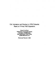
Figure 1: MMPP States of 2-Source Trac mean ri?1 . When in state i, cells are generated according to a Poisson process with rate i . The discrete-time version of MMPP is MMBP (Markov Modulated Binomial Process). It is a discrete-time m-state Markov chain, where the sojourn time for state i is geometrically distributed with mean qi?1 . When in state i, during each time slot, which is equal to the time of a cell arrival, one cell will arrive with probability pi , i.e. the cell generation process is binomial process. If we assume the trac model for one source is a two-state MMPP (MMBP), one state is silent and the other one is active with arrival rate i (with arrival probability pi ), we can still use the MMPP (MMBP) to model the aggregate trac from N sources. The number of states needed to model the aggregate trac will be 2N . This is shown in Figure 1. There is much research going on in this area, however, this is not the focus of our project. We need to choose one trac model for the simulation we need, as for the analytical tractability and scalability, we choose MMPP(MMBP) as our trac model.

2.3 Call Admission Control Schemes When a user needs to communicate, it will provide a connection setup request to the network. The request contains the parameters that describe the trac source characteristics, such as the peak cell rate, average cell rate, average burst length etc. The network switches then need to make a decision in real time. This requires that the computation involved be tractable [5].

6


In theory, it is possible to develop a Markovian model of a whole communication network and solve it numerically with the new connection in order to determine if the network can accommodate it or not. In practice, such a queuing model consists of hundreds of queues with trac generated from thousands of sources. It is impossible to solve such queuing models numerically in real time, even for small-sized networks, due to large storage and processing requirements. A well-known approach in queuing theory to analyze large queuing networks is to decompose the network into individual queues and analyze each queue in isolation. This method, although approximate for most cases of interest, has been used satisfactorily to obtain the performance metrics of various real systems [5]. But there is still another problem left. Will the nodes along the virtual path see the same trac? In other words, will the trac source characteristics be changed after going through some switches? In ATM networks, if a switch buer full and at this time if some cells arrive, they will just be dropped; so the trac can just become smaller than that at the source node. So the service process at one node will not be in uenced by the up-stream [5]. In the following, some popular Call Admission Control schemes will be surveyed. In the next section, we will present our Neural Network approach. As mentioned before, Call Admission Control is closely related to bandwidth allocation. What some of the schemes do is actually to calculate the bandwidth that should be allocated to the incoming source and the aggregate tracs already existing, plus the new incoming trac. If the the available bandwidth is greater than the bandwidth calculated, then the new trac will be accepted.

2.3.1 Peak Rate In peak rate multiplexing, each connection is allocated its peak bandwidth. Doing so causes large amounts of bandwidth to be wasted for bursty connections, particularly for those with large peak=average rate ratios. However, this Peak Rate Deterministic multiplexing can eliminate cell level congestion almost totally. This scheme is easy to implement, but due to the waste in resources, it is not a good one.

2.3.2 Equivalent Capacity The Equivalent Capacity scheme tries to nd the \equivalent capacity", which the trac source requires to satisfy the QoS requirement for each

7 connection. Then sum of all the equivalent capacities of each connection yields the total equivalent capacity. This sum may overestimate the required aggregate trac since interaction between individual connections is not taken into consideration. To capture the eect of multiplexing, the Gaussian approximation is used together with the equivalent capacities to determine the equivalent capacity of the aggregate trac [6].

3 The Neural Network Approach The purpose of our project is to predict in advance of transmission the Quality of Service (QoS) that will be obtained for a particular ATM call. The tool used in this prediction is a learning networks which will \observe" the behavior of the real system and store this information in the form of appropriate neural network weights. Assume that the only QoS criterion considered is the cell-loss ratio of ATM switches, which is indeed the most important criterion so that it is worth considering in its own right. What we want to achieve is to store the relationship between the cell loss ratio of aggregate trac, and the trac parameters, within a \small neural network". We use the Neural Network learning process to achieve this.

3.1 Neural Networks and Learning A neural network's ability to perform computations [17] is based on the hope that we can reproduce some of the exibility and power of the human brain by arti cial means. The basic processing elements of neural networks are called arti cial neurons. Neurons perform as summing and nonlinear mapping functions. In some cases, they can be considered as threshold units that re when their total input exceed certain bias levels. Neurons usually operate in parallel and are con gured in regular architectures. They are often organized in layers, and feedback connections both within the layer and toward adjacent layers are allowed. Each connection strength is expressed by a numerical value called a weight, which can be modi ed. From another aspect [17], neural networks can be considered as a class of mathematical algorithms since a network can be regarded essentially as a graphic notation for a large class of algorithms. What these algorithms to do is to store some information in the neural networks in the form of proper weights. The weights totally represent the information the neural network tends to store.

8

3. THE NEURAL NETWORK APPROACH

3.2 The Random Neural Network Model

Here we recall the Random Neural Network model which will be used in our [1, 2, 3]. The Random Neural Network is composed of a set of n neurons. Among the neurons, there are positive and negative signals circulating around. When a positive signal arrives to a neuron, the potential of this neuron increases by 1. However, when a negative signal arrives, the potential decreases by 1. When the potential of a neuron is greater than zero, the neuron can re. When it res, it emits one positive or negative signal, and at the same time, the potential decreases by one. Signals can also arrive from outside. All the arrival processes are Poisson processes, while the ring times are exponential [1]. We use = ((1); (2); : : : ; (n)) and = ((1); (2); : : : ; (n)) to represent the positive and negative signal arrival rate to each of the neurons from outside (n is the number of neurons), r = (r(1); r(2); : : : ; r(n)) to represent the ring rate when the neuron's potential is greater than zero. When a neuron i res, the probability that the signal goes from i to j is p+ (i; j ) or p?(i; j ) by positive or negative signal respectively. P The probability the signal goes out of the network is d(i). So d(i) + nj=1 p+ (i; j ) + p? (i; j ) = 1. We call w+ (i; j ) = r(i)p+ (i; j ) and w? (i; j ) = r(i)p? (i; j ) weights which represent how strong the connections are between the neurons. Let k(t) be the vector of neuron potentials at time t and k = (k1 ; :::; kn ) be a particular value of the vector. Let p(k; t) = Pr[k(t) = k] and p(k) denote the stationary probability distribution, i.e.

p(k) = tlim !1 Prob[k(t) = k] qi(t) is de ned as the marginal probability that neuron i is excited, i.e. qi (t) = Pr[ki(t) > 0]. Let q(t) = (q1 (t); q2 (t); : : : ; qn(t)). So q = limt!1q(t)

is the probabilities of steady state. Here we view and as inputs to the neural network and q as the outputs. The relationship between q and w+ (i; j ) and w? (i; j ) are de ned in Theorem 1. Theorem 1. [1] Let + qi = r(i)+ (i)? (i)

(1)

3.2 The Random Neural Network Model

9

Where the + (i) and ? (i) satisfy the following system of nonlinear simultaneous equations:

+ (i) =

X j

qj r(j )p+ (j; i) + (i)? (i) =

X j

qj r(j )p? (j; i) + (i) (2)

If a nonnegative solution + (i); ? (i) exists to equations (1) and (2) such that each qi < 1, then

p(k) =

n Y i=1

[1 ? qi]qik

(3)

i

The quantity we are most interested in here is q. We can view the de nition of q as q = f (q) = (f1 (q); f2 (q); : : : ; fn (q)), where fi (q) = + (i)=(r(i) + ? (i)). We have been using the following x-point method to obtain the numerical solution of the nonlinear equations (1) and (2).

(

q(0) = (0; 0; : : : ; 0) q(k+1) = f (q(k) )

(4)

This method, which has been used systematically in recent years, works quite well in dierent kinds of circumstances. We have proved that this x-point method converges by showing the following: The function f is a map-in function in [0; 1]n Rn, i.e. f (q) 2 [0; 1]n for 8q 2 [0; 1]n , under some conditions which can be always satis ed by monitoring the \inputs" ( and ) to the neural networks. Let J be f 's Jacobian matrix. There exists a matrix J 0 similar to J and a constant c < 1 such that kJ 0 kinf c < 1. So J and J 0 have the same eigenvalues and the spectral radius of J 0 (J 0 ) c < 1. Then we have (J ) c < 1, from which we know that there exists a norm k k such that kJ k c < 1. So f is a \contraction". From Theorem 2, we have that the itheration de ned by (4) will converge to a unique xed point q 2 [0; 1]n .

Theorem 2. [4] Let B : Rn ! Rn be a contraction on some closed set S Rn such that B (x) 2 S for x 2 S . Then B has a unique xed point x 2 S . Furthermore, if c < 1 is the contraction constant, and xk = B (xk ) with x 2 S , then all Xk 2 S , and kxk ? x k [c=(1 ? c)]kxk ? xk? k. 0

+1

1

10


3.2.1 Learning

The purpose of a neural network is to \learn". What we want to do is to train the neural network in order to achieve some desired input/output relationship, which is de ned by the following vectors: = ((1) ; (2) ; : : : ; (m) )

= ((1) ; (2) ; : : : ; (m) ) Y = (Y (1) ; Y (2) ; : : : ; Y (m) )

where m is the number of training pairs.

(k) = ((k) (1); (k) (2); : : : ; (k) (n))

(k) = ((k) (1); (k) (2); : : : ; (k) (n)) Y (k) = (Y (k) (1); Y (k) (2); : : : ; Y (k) (n))

and Y (k) is the desired output vector under the inputs (k) and (k) . Let Q(k) be the output of the neural network under the input vector (k) and (k) . The training will modify the weight matrix in order to make the dierence between Y (k) and Q(k) as small as possible. The training algorithm [3] is based on a gradient descent method to minimize the following cost function:

Ek = 21

n X i=1

ai (qk (i) ? yk (i))2 ; ai 0

The rule for weight update may be rewritten as

wk (u; v) = wk?1 (u; v) ?

n X i=1

ai (qk (i) ? yk (i))[@qi =@w(u; v)]k

where wk can be w+ or w? and > 0 is some constant.

3.3 The Neural Network Approach

Let us discuss some of the bene ts of the Neural Network Approach. First, this approach can t any trac model, or even avoid any assumption of a trac model. However, the existing equivalent bandwidth and the fast buer reservation approaches depends on the trac model they choose [6, 8]. If

3.3 The Neural Network Approach

11

the trac model is proved to be unrealistic, then the approach would be invalid. Actually, the neural network approach will be implemented using on-line collected user data. Even if under some trac model (assume this model is realistic), the Neural Network approach can achieve more accurate prediction because it is based on real data collection. The admission decision made by existing methods such as equivalent capacity [6] is based on the calculation of equivalent bandwidth and the calculation inevitably involves some approximation. For example, the equivalent bandwidth scheme [6] is based on a renewal process. Solving the aggregate trac will involve many states ( 2N where N is the number of trac sources), assuming two-state ON/OFF MMPP or MMBP model for each source. However, the calculation must be done in real time. Thus the Equivalent Bandwidth approach actually calculates the equivalent bandwidth of a single source, then uses a Gaussian Approximation to derive the approximate aggregate bandwidth. Tabling is an approach often used in the network area and one could make use of tabling here. We could use o-line simulation, based on the MMPP for example, to build up a table. Each entry gives the equivalent bandwidth of the aggregate trac speci ed by the trac parameters (such as the number of trac sources, peak rate, average rate, burst length). However, the table has to contain all the possible trac parameters, which will make the table tremendously large. Table look-up will then be very time and space consuming. Actually there is some relationship between the table entries. For example, the bigger the average rate is, under the same peak rate, the bigger the equivalent bandwidth will be. If there is a way to \condense" the table, i.e. to store the information in a \compacted" way, it will improve the situation substantially. The neural network approach follows this approach. In the following, we will introduce the Neural Network approach in detail. The basic idea is to store a large amount of information within a \small" neural network. The neural network stores the information in the form of a weight matrix and the learning process is used to obtain this weight matrix. The information we want to store in the Neural Network is the relationship between the trac parameters (the number of trac sources, peak rate, average rate, burst length), switch architecture (switching rate and buer capacity) and the cell-loss ratio. To achieve the desired weight matrix, we need representative data. We will use the data collected from real trac. However, as the starting step, we need to test the feasibility of this neural

12


network approach and we use simulation, which is based on some speci c trac model, to collect the data. Later on, if neural network approach were adopted in real industry, the data collection process should be done in real communication network operating circumstances.

3.4 The Simulation Model Since we will use MMBP model, we consider that a discrete time simulation will t best [20, 21]. The time axis is divided into equal intervals called slots. As cells arrive, they are stored in a xed size buer. Transmission (service) of a cell is synchronized to start only at slot boundaries. Cells which arrive in a slot are eligible for transmission at the beginning of the next slot. If cells arrive when a buer is full, they will be lost. Each node has several incoming sources of cells. We assume they are independent of each other and each source has the same pattern. Note that for each switch in the network, the incoming link speed may be dierent from that of the outgoing link. So the arrival cell slot length is dierent from the departure cell slot length. The simulation has to take care of this. The simulation parameters are the number of trac sources (N ), the peak rate (p), the average rate (m), the burst length (ton ), the buer size (B ), the outgoing link rate (R). The data we want to collect is the cell loss ratio under these parameters. Here we use the incoming link rate over the outgoing link rate as p, i.e. a relative peak rate. The same for average rate, i.e. m is the average arrival cell rate over outgoing link rate. The burst length (ton ) is in the units of outgoing link cell slot. The related parameters for each trac source, a and b (de ned in Section 2.1), are determined by the relationship shown in Section 2.1. We simulate the network trac using the model described above. We want to see how the cell-loss ratio changes with values of the parameters. Figure 2 shows the relationship between average rate (with other parameters xed) and cell-loss ratio. Figure 3 shows the relationship between burst length and cell loss ratio. Figure 4 shows the relationship between the number of sources and loss ratio. The simulation is just a starting point from which the Neural Network will \learn" and predict the cell-lose ratio.

3.4 The Simulation Model

13

#sources = 4, peak−rate = 0.9, aburst−length = 30 0.16

0.14

Cell Loss Ratio

0.12

0.1

0.08

0.06

0.04

0.02

0 0

0.05

0.1

0.15 average−rate

0.2

0.25

0.3

Figure 2: Cell Loss Ratio vs. Average Rate

#sources=4, peak−rate=0.6, average−rate=0.16

−3

3

x 10

2.5

Cell Loss Ratio

2

1.5

1

0.5

0 0

5

10

15

20

25 30 Burst Length

35

40

45

50

Figure 3: Cell Loss Ratio vs. Burst Rate

14

3. THE NEURAL NETWORK APPROACH peak−rate = 0.9, average−rate = 0.04, burst−length = 30 0.2 0.18 0.16

Cell Loss Ratio

0.14 0.12 0.1 0.08 0.06 0.04 0.02 0 0

5

10

15 # Sources

20

25

30

Figure 4: Cell Loss Ratio vs. Number of Sources

3.5 Prediction by the Random Neural Networks Usin our simulation, we obtain a set of data, which will represent the relationship between the trac parameters and cell loss ratio. We then use the Random Neural Network learning process to store the information in the network's weight matrices.

3.5.1 Input Output Relationships We have N , p, m, ton, B as the inputs to the neural network and the cell loss ratio as the output. We represent the outputs of the neural network by a vector y = (y1 ; y2 ; : : : ; yn ), where yi is 1 or 0 and represents the cell loss ratio's order 10?i . Ideally, at most one of the yi s should be 1. In order to reduce the size of the neural network to make the training easier, we set up dierent Neural Networks for dierent loss ratio requirements. The training data will be dierent for each of the neural networks. Now we have m neural networks. Each of the neural networks has two outputs, one of them represents that the loss ratio is bigger than the order 10?i , the other one represents that the loss ratio is equal to or lower than the order 10?i . One and only one of them should be 1. For the same inputs, the outputs of each neural network will clearly be dierent from each other. 0

3.5 Prediction by the Random Neural Networks

15

4 8 1 5 9 2 6 10

3 7

Figure 5: Neural Network Topology

3.5.2 Random Neural Network Architecture (Topology) The topology we choose for the Random Neural Network is directly related to the training eect. For a speci c problem, we should choose a suitable Neural Network topology. How to choose a topology is not yet a standard procedure, so we need to proceed via many experiments. However, there is still something there we can turn to. For example, if only one of the neural network outputs is 1 and the others are zero, then the topology which is graphically shown in Figure 5 will be quite helpful. The overall topology is feed-forward. However, the connections among the output layer neurons are recurrent. In such a topology, the output neurons compete with each other and the \strongest" one will dominate and will give the \biggest" output, here 1. The others will be \pushed" down and will give \small" outputs, here 0. This just suits the structure of our training data among whose outputs there is only one \1" and the others are \0". This output layer topology is called a competitive network, which is motivated by what is believed to be a mechanism used in the brain in areas like the visual cortex of the brain. The mathematics behind it could be approached by writing the equations for the neural outputs in terms of a set of coupled nite dierence or dierential equations, depending on the kind of neural network used and whether it is discrete time or continuous. The weights serve as coecients for the set of dierence equations describing the neurons in a competitive arrangement. Using classical analysis, it may

16


be shown that under certain conditions the system will evolve to a stable equilibrium, which is the state in which all the neurons have shut o except for the winning neuron, which saturates at its maximum output."

3.5.3 Comparison with other Neural Networks For the connectionist model, the famous learning algorithm is the backpropogation algorithm which works well for feed-forward networks. Only under certain special conditions can it be used in recurrent networks, i.e. those which contain feedback. However, the neural network topology shown in our last section, which is recurrent, ts the output structure of our problem particularly well. Thus the Random Neural Network Learning algorithm [3], which covers both feedforward and recurrent topologies, allows us to handle the case we are interested in with ease.

3.5.4 Training Results In this section, we show how well the trained Neural Network can serve the needs of the CAC function. After the RNN is trained using the simulation data, we feed new trac data into the neural network and compute the outputs of the RNN, which predict cell loss ratio. The prediction is compared with the new observed simulation results in Figure 6. The explanation is provided below. Draw a vertical line across Figure 6, the intersect point on the rst line shows the peak cell arrival rates, the point on the second line shows the average cell arrival rates, the point on the third line shows the burst length and the point on the last line shows the prediction result under the inputs indicated by the rst three points. The value of \2" or \-2" of the last line means that the prediction is a correct prediction. \2" means the prediction leads to a correct \admission", while \-2" means the prediction leads to a correct \Rejection". \-1" means that the prediction will lead to a wrong \Admission", which means that the wrongly \admitted" trac will suer cell loss ratio greater than the QoS requirement and at the same time other trac will also suer from this wrong decision, because here we consider the aggregate trac. \1" means that the prediction will lead to a wrong \Rejection" and the trac has to call some other path. We can see that the prediction is correct 85% of the time. If we consider the \1" decision is \half right", then the proportion of correct decision is

3.6 Use in the ATM Network Switch

17

Prediction after Learning (# of traffice sources = 30) 10 peak rate

Prediction Results and Input Parameters

8 average rate 6

average burst length

4 prediction after learning 2

0

−2

−4 0

20

40

60

80 100 120 Training Pair Index

140

160

180

200

Figure 6: 90%.

3.6 Use in the ATM Network Switch Using the Neural Network approach, the ATM switch can make the admission decision without calculating the equivalent bandwidth. The time to make the decision is just the time to calculate the output of the Neural Network under the user's speci ed trac parameters, which is very fast. However, if the switch needs to calculate the equivalent bandwidth for other management purposes, it could be done after the call admission, as part of the \background" work of the switch. If the new incoming trac is correctly admitted, then the equivalent bandwidth of the aggregate trac is certainly lower than the available link rate. From the above discussion, we know that the inputs to the neural networks are p (peak-rate/link-rate, here the \link-rate" can be considered as the equivalent capacity), m (average-rate/link-rate), ton (burst length in cell time of the incoming link). Now we reduce the link rate by half, so the inputs to the neural network will be 2p, 2m, 2ton . If the cell-loss ratio still lower than the QoS requirement, then we know the equivalent capacity is

18

REFERENCES

still lower than the link-rate/2, we can reduce the bandwidth by half again to test. Now if the loss ratio is higher than the requirement, then we know the equivalent capacity is higher than link-rate/2, we then increase it by half. So the inputs now will be (4=3)p, (4=3)m, (4=3)ton . This process can be repeated until we nd the required equivalent capacity range. If this process starts from the equivalent bandwidth before admitting this new trac, it will take less time. When a connection terminates, we can also use the above \computation" to get the equivalent bandwidth.

4 Future Work In this work we have observed that a Random Neural Network can achieve correct predicton rates of 85 ? 90%. It is important to improve the training in order to get better prediction. Thus the rst thing to do in the future is to improve the learning algorithm in order to achieve perfect learning. We also need to use the data collected from real trac for training and then proceed to on-line training. For implementation in industry, we need to consider setting up a group of neural networks instead of a single one, which would be resident in the switch. Each one of them would be responsible for a subset of the requirements, so that dierent neural nets would be in charge for dierent loss-ratio requirements.

5 Acknowledgment Thanks for Dr. Raif O. Onvural, my teacher in the \Network Design and Analysis" class. Both during and after class, he answered many of my questions concerning ISDN and ATM. Also thanks to Prof. Don Rose and Xiaobai Sun for their support and encouragement during the nonlinear xedpoint proof. Thanks for Xiaobai's patient discussions with me. Thanks for Dr. James Murrell for helpful suggestions and discussions. Finally, thanks to Prof. Erol Gelenbe, my advisor, for his patience and advice throughout this project.

References [1] Erol Gelenbe, Random Neural Networks with negative and positive signals and product form solution, Neural Computation, 1(4), 1989, pp.

REFERENCES

[2] [3] [4] [5] [6] [7] [8] [9] [10] [11] [12] [13] [14]

[15]

19

502-510. Erol Gelenbe, Stability of the Random Neural Network Model, Neural Computation, 2(2), 1990, pp. 239-247. Erol Gelenbe, Learning in Recurrent Random Neural Network, Neural Computation, 5, 1993, pp. 154-164. Don J. Rose, Numerical Analysis Class Notes, pp. 250 - 258. Raif.O. Onvural, Asynchronous Transfer Mode Networks': Performance Issue, Artech House, 1993. L. Gun, R. Guerin, A uni ed Approach to Bandwidth Allocation in High-Speed Networks, INFORCOM'92, Italy, 1992, pp.1-12 . P.Joos, W. Verbiest, A statistical Bandwidth Allocation and Usage Monitoring Algorithm for ATM Networks, ICC'89, 1989, pp.415-42. J.S.Turner, Managing Bandwidth in ATM Networks with Bursty Trac, IEEE Network, 1992, pp.50-58. B.G.Kim, P.Wang, ATM Network: Goals and Challenges, Communications of the ACM, Feb. 1995, Vol.38, No.2, pp.39 - 44. Ronald J. Vitter, ATM Concepts, Architectures, and Protocols, Communications of the ACM, Feb. 1995, Vol.38, No.2, pp.30 - 38. G.D. Stamoulis, Trac Source models for ATM networks: a survey, Computer Communications, Vol. 17, No.6, June. Jaime Jungok Bae, Tatasuya Suda, Survey of Trac Control Schemes and Protocols in ATM Networks, Proceedings of the IEEE, Vol.79, No2, Feb. 1991, pp.170-189. ATM User-Network Interface Speci cation, PTR Prentice Hall, 1993. L. Gun, Gerald A. Marin, An Overview of the ATM forum an the Trac Management Activities, Asynchronous Transfer Mode Networks, Edited by Y. Viniotis and R.O. Onvural, Plenum Press, New York, 1993, pp.2129. Douglas S. Holtsinger, Congestion Control Mechanisms for ATM Networks, Asynchronous Transfer Mode Networks, Edited by Y. Viniotis and R.O. Onvural, Plenum Press, New York, 1993, pp. 107-122.

20

REFERENCES

[16] Khosrow Sohraby, Highly-Bursty Sources and Their Admission Control in ATM Networks, Asynchronous Transfer Mode Networks, Edited by Y. Viniotis and R.O. Onvural, Plenum Press, New York, 1993, pp.123133. [17] Jacek M. Zurada, Arti cial Neural Systems, West Publishing Company, 1992. [18] William Stallings ISDN, An Introduction, Macmillan Publishing Company, 1989. [19] Gary C. Kessler ISDN, McGraw-Hill, Inc., 1990. [20] Herwig Bruneel, Byung G. Kim, Discrete-Time Models for Communication Systems Including ATM, Kluwer Academic Publishers, 1993. [21] I. Mitrani, Simulation Techniques for Discrete Event Systems, Cambridge University Press, 1982.