Dynamic Cellular Manufacturing System Design for

Journal of Production Research & Management eISSN: 2249-4766, pISSN 2347-9930 Volume 4, Issue 2 www.stmjournals.com

Dynamic Cellular Manufacturing System Design for Automated Factories P. Narendra Mohan1*, Ch. Srinivasa Rao2 1

Dept. of Mechanical Engineering, Acharya Nagarjuna University, A.P, India 2 Dept. of Mechanical Engineering, Andhra University, A.P, India

Abstract In this paper, an integrated mathematical model of the multi-period cell formation in a dynamic cellular manufacturing system (DCMS) is proposed with the aim of getting the optimal cost f o r i t . In DCMS, the formed cells in the current period may not be optimal for the next period, so the reconfiguration of the cell is needed, thus we have a tendency to use DCMS. The paper examines the influence of the trade-off between assorted manufacturing costs on the reconfiguration of the cells in Cellular Manufacturing System (CMS) under a lively environment and the proposed model is implemented to a wide range of numerical examples.

Keywords: Dynamic cellular manufacturing system, reconfiguration, alternative routing, production planning *Author for Correspondence E-mail: [email protected]; [email protected]

INTRODUCTION Production planning and control procedures have been simplified by Wemmerlov and Johnson [1] with the use of cellular manufacturing (CM). Obvious benefits gained from the conversion of the shop are less travel distance for parts, less space required, and fewer machines needed. Since like part types are grouped, this could lead to a drop in setup time and allow a quicker response to changing conditions. CM is a hybrid system linking the advantages of both job shops (flexibility in producing a wi de var i et y of products) and flowlines (efficient flow and high production rate). In CM, machines are located in close proximity to one another and dedicated to a part family. This provides the efficient flow and high production rate similar to a flow line. The use of general purpose machines and equipment in CM allows machines to be changed in order to handle new product designs and product demand with little effort in terms of cost and time. So it provides great flexibility in producing a variety of products. Rheault et al. [2] for the first time introduced the concept of Dynamic Cellular Manufacturing System (DCMS) to overcome the limitations of the traditional CMS. If any change in the product demand occurs, CMS

ignores the product restructure and various other factors. In CMS the product mix and part demand is stable in the entire planning perspective. DCMS is related to reconfiguration of manufacturing cells including part families and machine groups at each period. Reconfiguration involves swapping the existing machines between each pair of cells, called machine relocation, adding new machines to cells including machine replication, and removing the existing machines from cells. Dynamic cellular manufacturing is used in environments where product demand is unstable, and the workstations in the facility can be easily rearranged. Most production environments involve changes in operating parameters, such as the product demand over time. In such a case, managing the production resources and balancing them between successive time periods with the aim of minimizing the production costs is known as “production planning (PP).” The aim of a standard PP problem is to minimize the total productionrelated costs, such as flexible production costs, inventory costs, and scarcity costs, over the fixed planning horizon. The main restrictions

JoPRM (2014) 12-30 © STM Journals 2014. All Rights Reserved

Page 12

DCMS Design for Automated Factories

of the PP problem are as follows: (1) inventory the preceding period, production quantity, and demand quantity and (2) Volume constraints which ensure that the total amount of work for every single resource (labour, machine, etc.) does not surpass the capacity in each period Kim and Kim [3]. Background of the Study In DCMS, the length of the planning horizon directly depends on the nature of the product. For example, if we encounter the seasonal products, like clothing or heater/cooler equipment, the planning horizon may consist of two six-month periods or four three-month periods. The DCMS is associated to reconfiguration of manufacturing cells together with part families and machine groups at each period. Reconfiguration involves trade off the existing machines between each pair of cells, called machine relocation, adding new machines to cells including machine replication, as well as removing the existing machines from cells. A schema of cell reconfiguration in DCMS for two consecutive periods is schematically shown in Figure 1. The system contains of two modern cells for each period. Because of the processing requirements, machine 3 must be relocated from cell 1 to 2 and machine 7 from cell 2 to 1 at the beginning of period 2. Also,

Mohan and Rao

machine 8 must be added to cell 2 at the starting of period 2 despite the fact that machine 1 will not be used during period 2. In this context, either machine 1 is kept in the same cell or moved to another cell because of the cell size restriction. Bearing in mind the utmost cell size is equal to 4, machine 1 moves to the outside of cell 2 and machine 8 is replaced by that. Thus, the above reconfiguration requires three machine relocations. In DCMS, the decision maker (DM) needs to identify how big the changes of the cell arrangement from a period to another are. As it is pointed out earlier, these changes are caused by fluctuations in the fabrication and outsourcing needs. In this condition, the DM has to formulate a suitable decision sandwiched between the available alternatives, such as adding up a new machine, relocating the equipment between present cells, outsourcing a few parts in addition to hiring/sacking the workforce, to maintain a balance between production and outsourcing costs. Taking such a decision can be crucial and perilous in the cost-intensive production systems, such as DCMS, for the reason that it can extensively influence the cell arrangement throughout the specified horizon planning. For this reason, the current paper describes the effect of the trade-off between production and outsourcing expenditure on the reconfiguration of cells in DCMS.

Fig. 1: A Schema of the Cell Re-confirmation in DCMS.


Page 13

Journal of Production Research & Management Volume 4, Issue 2 eISSN: 2249-4766, pISSN 2347-9930

Material handling is the most significant operational characteristic of CMS. In reality, material handling price in the CMS is separated into two major groups: inter and intracellular movements. It is an uncommon way to find several preceding jobs, taking into consideration both inter and intra-cell movements in the DCMS concurrently, particularly, taking into account the process series. Among the researches associated to the DCMS, only Wicks and Reasor [4], Defersha and Chen [5], Safaei et al. [6] and Safaei et al. [7] considered the operation sequence for intercellular travels. Added advantage of the research by Safaei et al. [7] considered the intracellular and intercellular travels by assuming the operation sequence. In the midst of the earlier studies Sankaran and Kasilingam [8] formulated an integer programming model which uses a stepwise linear purpose to characterize the cost of intracell moves. Ranges of cell sizes, in terms of the number of machinery enclosed in a cell, are defined. As cells turn into outsized and drop into the next range, there is a stepwise raise in the cost of an intra-cell move though their model does not consider the impact on which demand variability may have on the system. Figure 2 shows the direct effects of the operation series on material handling. For instance, operations 1 and 3 of part 11 must be done on machine 7 in cell 1. Furthermore operation 2 must be done on machine 5 in cell 2. As a result, to watch the operational series, the processing route for part 11 requires two

intercellular movements as of cell 1 to 2 as well as vice-versa. With the like cause, the processing route intended for part 3 in cell 2 requires two intra-cell movements. From the effectiveness point of view, in view of both intercell and intracell material handling at the same time causes a steadiness in the size of the formed cells. The cause is that extremely large cells engage high intracell and low down intercell material handling costs. On the other side, very little cells engage high intercell and low intracell material handling costs. To simplify, as shown in Figure 3, it is supposed that the part varieties are shifted inside cells by an automaton or manpower and between cells by a conveyor, crane, truck, or Automated Guided Vehicle (AGV). Here the, inter-cell movements are handled by means of manpower within cell 1 furthermore with an automaton in cell 2. Perceptibly, in this situation, the capacity and unit cost of the intracell movement are a lesser amount than the associated cost incurred by means of intercell movement. In this paper, the authors broaden the original model projected by Safaei et al. [9] with a new involvement on the outsourcing by means of taking into account of the carrying inventory, backorder, and partial outsourcing. The planned model is capable to form the optimal cells and to determine the most advantageous alternate arrangement (i.e., production or partial (or) full outsourcing) for every part type at every period throughout the specified horizon planning Safaei et al. [9].

Fig. 2: Effect of the Operation Sequence on Inter/Intra-cell Material Handling.


Page 14


Mohan and Rao

Fig. 3: Hypothetical Layout with Nearly Same Distance between Each Pair of Machines and Cell Locations. Four objectives are considered to minimize in the proposed model as follows: (1) Machine costs consist of the constant and variable costs. (2) Material handling costs consist of inter and intracell movement costs by considering the operation sequence. (3) Cell reconfiguration cost consists of the machine relocation costs. (4) Outsourcing costs consist of the inventory carrying, backorder and subcontracting costs.

LITERATURE REVIEW The concept of DCMS was first introduced by Rheault et al. [2]. Previous investigations Harhalakis et al., [10], Vakharia and Kaku [11] have been done in the context of modeling and methodology of the cell formation problem in dynamic environment by assuming stable cells, i.e., without cell layout change. Harhalakis et al. [10] applied a twostage design approach to obtain a cellular design with the minimum expected intercell movement cost over a system design horizon which was broken down into elementary time periods. In the first stage, a bottom-up aggregation procedure to minimize the “normalized inter class traffic” is proposed. In the second stage, a procedure is presented to attempt further improvement, in which the significance of a machine to a cell is validated. Vakharia and Kaku [11] incorporated longterm demand changes into their 0–1 mathematical programming cell design method by reallocating parts to families to regain the benefits of cellular manufacturing systems. Similarly, new parts are allocated to existing cells. So, cells are not rearranged in

their multiperiod design. They identified three redesign strategies: (1) part reallocation, (2) partial cell system redesign, and (3) complete cell system redesign. Using the first strategy, parts may be reallocated to other cells and some additional equipment may be purchased to meet increased processing loads but the composition of cells in terms of machine types is not altered. In the second and third strategies the composition of cells in terms of machine types is also changed. Their study only models the first strategy. An integer model is presented for this strategy and a solution procedure is developed. The authors restrict parts that can be reallocated to only those with demand changes. The reason given for this is to minimize tooling costs although the costs of tooling are not considered by the paper’s model. The model does not consider production cost that is based on the size of the cell but does include a constraint that limits the number of machines that can be assigned to a cell. A wide-ranging review of the DCMS literature can be originated in Safaei et al. [7] and Balakrishnan and Cheng [12]. PP in the CMS was discussed in Chen [13] and Olorunniwo [14]. Reconfigurable layouts also addressed by Benjaafar and Sheikhzadeh [15] and Vakharia et al. [16]. In addition, the flexible layouts to accommodate the dynamic demand have been discussed by Venkatadri et al. [17] and Askin et al. [18]. A variety of well-organized methods were developed to examine and solve the cellular manufacturing problems. These take account of the traditional mathematical programming Chen [19],Heragu and Chen [20] and simulation studies Shang and


Page 15


Tadikamalla [21],Shinn and Williams[22]. Petrov [23] was the first who noted that a redesign of the PP and scheduling system is compulsory when implementing cellular manufacturing principles to production systems. He considered various types of flow line cells that can be constructed by means of group technology and determined the planning conditions that are required to get better both the performance of these cells and the performance of the whole system consisting of interconnected cells. Hyer and Wemmerlo¨v [24] projected a common structure for PP and control and applied this framework to CMS in order to produce components or parts. Their framework is a hierarchical decision procedure that consists of three stages: (1) decide at what time and in what quantities final goods are to be produced; (2) find out what parts are to be produced through a definite time period as well as in what quantities; and (3) determine at what time and in what order jobs (i.e., parts) have to be processed at a range of workstations. Dale and Russell [25] reported on distinctive production control problems, such as load balancing problem, in flow line CMS. The cells consist of various types of machines and operators who often are not equally capable. In such configurations, it can turn out to be a difficulty to maintain a good balance between key machine use and worker utilization. Fluctuations in the product mix and volume and introduction of new products can make too much of these troubles. Redesigning the production system itself to explain these troubles is not often possible or good enough, so the production control system has to deal with these problems. The same system holds for the problems caused by the allocation of key machines between cells. In these cases, the recognition of the complete potential of a CMS depends mostly on the PP and control system design. Wemmerlov [26] addressed the problem how to exploit the advantages of cellular manufacturing in a Material Requirement Planning (MRP) system. The gain of producing like parts in one cell should be

predictable and handled by the MRP system in order to achieve the benefits of CMS. Askin and Mitwasi [27] designed a mathematical model to put together a number of decisions in setting up a manufacturing system that consists of selecting a manufacturing technology for every product type (process selection), identifying utmost production levels of every product type (capacity planning), and locating production resources and routing of products to requisite resources (facility layout). They showed the applicability of the proposed approach by distinguished between the proposed integrated approach and the hierarchical approach. Habich [28] developed a PP framework that recognizes the essential planning problem resulting from giving planning autonomy to cells that are interconnected in their main production process. He viewed the essential problem of the central planning level to produce an overall best possible from the various local optima that were generated by the decentralized planning of the cells. His move towards the central planning is to consider the set of orders that necessitate succeeding process in different cells, determine for these orders suitable sequences between the cells and designed throughput times per cell (e.g., order due dates), such that the cells will be able to finish these instructions within their due dates while at the alike time enough flexibility is accessible to optimize the planning in the cell. Rohloff [29] developed a framework that decentralizes setting up to the cells (as autonomous units) as much as possible. The framework places a strong highlight on the horizontal coordination level, e.g., the direct coordination between different autonomous units. The vertical coordination levels can be considered as an attempt to solve certain remaining planning problems using a hierarchical approach. Banerjee [30] proposed a tactic for the design of an integrated manufacturing planning and control system to a real-life CMS. Schaller et al. [31] proposed a two-stage approach named CF/PP for integrating the cell formation and PP in a CMS. In the primary


Page 16


stage, a list of potential cells is identified to minimize the production costs and holding/backorder costs over the planning horizon. In the secondary stage, using all the on top of information in terms of part-related costs, equipment capacities and the like as well as the list of the obtained potential cells in the first stage, the ‘‘best’’ set of cells are selected and a production plan for each part over the planning horizon is identified simultaneously. Chen and Cao [32] proposed an integrated model for PP in a CMS that minimizes the inter-cell material handling cost, fixed charge cost of setting up manufacturing cells, cost of holding the completed items over the planning horizon, cost of setting up the system to process dissimilar parts in different time periods, and machine operating cost. They developed a heuristic method to solve the presented problem. They first changed the proposed model into an equivalent problem of the reduced size with an entrenched suboptimization problem. Then, they used a tabu search procedure to search for the optimal solution of the transformed problem. Defersha and Chen [5] proposed a mathematical model for the design of CMS. It incorporates a dynamic cell configuration, alternative routings, and operation sequence, multiple units of the same machines, machine capacity, and workload balancing among cells, operation cost, subcontracting cost, tool consumption cost, setup cost, and other practical constraints. In a similar study, they also proposed a wide-ranging mathematical model for the design of a DCMS based on tooling requirements of the parts and tooling available on the machines. The model incorporates a dynamic cell configuration, alternative routings, lot splitting, operation sequence, multiple units of identical machines, machine capacity, workload balancing among cells, operation cost, cost of subcontracting part processing, tool consumption cost, cell size limits, and machine adjacency constraints, Defersha and Chen [33] and Nomden and Van der Zee [34] addressed the way mid-term investments in process planning, machines, and secondary resources to improve the shop performance in a Virtual Cellular Manufacturing (VCM). Their most important

Mohan and Rao

focus is on an increase of routing flexibility in terms of the number and distribution of alternative machines available for a product family, and the number of secondary resources. The obtained results show that (1) a small number of alternative routes will mostly be adequate, (2) a chained distribution of routes is preferable, and (3) secondary resources are relevant only under specific conditions. Ioannou [35] developed a comprehensive method for transforming pure functional manufacturing shops into hybrid production systems that include both cellular and functional areas. In this study, the facility redesign approach first derives the layout of the work centers within each cell and then places the cells within existing departments according to a time-phased implementation plan. The incremental cell implementation is dictated by funds constraints that limit the allowable investment in each fiscal period. The aspiration is to make best use of the net benefit from cell implementation, expressed as the difference between the savings in material handling effort and the cost of machine rearrangement. Recently, Kioon et al. [36] proposed an integrated approach to CMS design, where PP and system reconfiguration decisions are incorporated in the presence of alternate process routings, operation sequence, duplicate machines, machine capacity and lot splitting. They formulated the problem as a mixed integer non-linear program and verified the model using some random small/mediumscale problems. Though, they have not discussed about the effect of the considering PP on the reconfiguration as the most challenging issue in DCMS. Actually, we want to show the DM may deviate from the optimum solution if the stability of the cell configuration during a multi-period horizon planning is considered as a subjective criterion.

PROBLEM FORMULATION This section covers the development of a multicriteria nonlinear mixed-integer mathematical model for the dynamic cell formation problem. The model incorporates real-life parameters like alternate routing,


Page 17


operation sequence, duplicate machines, product mix, product demand, batch size, processing time, machine capacity, and various cost factors. The guiding framework adopted in this model was developed initially by Mungwattana [37], Tavakkoli et al. [38], and Safaei et al. [9]. The objective of the proposed model is to minimize the sum of the machine constant cost, the operating cost, the intercell material handling cost, and the intracell material handling cost for the given period. The proposed model is expected to satisfy the following: 1. Establishing the part families and machine groups simultaneously. 2. Determining the optimum number of cells in each period (cell size). 3. Determining the optimal alternative process plan for each part in each period (alternative process plan). 4. Determining the number of machines needed for each type in each period (machine duplication). 5. Adding, removing or relocating machines in c e l l s between each two consecutive periods as required (machine relocation). 6. Considering the inter- and intra-cell material handling with the different batch type for each part. 7. Considering the machine capacity and maximal cell size. Assumptions The following assumptions are made for the development of the model. 1. Each part type has a number of operations that must be processed according to a known sequence. The sequence of operations enumerates from 1 in an ascending order. 2. The processing time for all operations of a part type on different machine types is known and deterministic. 3. The demand for each part type in each period is known and deterministic. 4. The capabilities and capacity of each machine type are known and constant over the planning horizon. 5. The cost of each machine type, also known as constant cost, is constant and known. This cost is independent of the

6.

7.

8.

9.

10.

11.

12.


workload allocated to a machine and it indicates the rent, overall service, maintenance, and other overhead costs [33]. This cost is also considered for each machine for each cell and period irrespective of whether the machine is active or idle. The variable cost of each machine type is known. The variable cost implies operating cost that is dependent on the workload allocated to the machine. The relocation cost of each machine type from one cell to another between periods is known. This cost consists of removal, shifting, and installation costs, where installation and removal costs are assumed to be same. If a new machine is added to the system, we have only the installation cost. On the other hand, if a machine is removed from the system, we have only the removal cost. To reduce the number of parameters of the system, we assume that the unit adding/ removing cost is a half of the relocation cost. Parts are moved between and within cells as batch. As mentioned earlier, inter and intracell batches related to the part types have diﬀerent sizes and costs. The reason is that in reality, the parts have different shape and size. For reducing complexity of t h e mo d e l , u n i t intercell and i n t r a ce l l movement costs are constant for all moves regardless of the distance travelled. Holding and backorders inventories are allowed between periods with known costs. Thus, the demand for a part in a given period can be satisfied in the preceding or succeeding periods. The maximum number of cells must be specified in advance and it remains constant over time. Each machine type can perform one or more operations (i.e., machine flexibility) without incurring a modification cost In other words, all machine types are assumed to be versatile machines. Partial subcontracting is allowed. It means that the total or portion of the demand of the part types can be subcontracted at each period. Also, the time-gap between releasing and receiving orders (i.e., lead time) is known in advance.

Page 18


Indices: c m p j h

= = = = =

Mohan and Rao

index for manufacturing cells (c = 1,…,C) index for machine types (m = 1,…,M) index for part types (p = 1,…, P) index for operations required by part p (j = 1,…,Op) index for time periods (h = 1,…,H)

Input Parameters: P number of part types Op number of operations for part type p M number of machine types C maximum number of cells that can be formed H number of periods Dph demand for part type p in period h tjpm processing time required to process operation j of part type p on machine type m 1, if operation j of part type p can be done on machine type m; ajpm 0, otherwise. Intra batch size for intra-cell movements of part type p βp Inter βp batch size for inter-cell movements of part type p γpinter intercell material handling cost per batch γpIntra intracell material handling cost per batch. For justification of CMS, it is assumed that (γintra/βpintra) < (γinter/βpinter) for all p αm amortized cost of machine of type m per period . βm Operating cost of machine type m for each unit time. In this work, a unit time of 1 h is used. δm Relocation cost of machine type m including installing, shifting, and uninstalling Tm Time-capacity of machine m in terms of unit time (hours) for each period. UB Maximal cell size, i.e., maximum number of machines per cell Decision Variables: Nmch number of machines of type m assigned to cell c in period h + Kmc number of machine type m added in cell c in period h Kmc − number of machine type m removed in cell c in period h Xjpmch 1, if operation j of part type p is done on machine type m in cell c in period h; 0, Other wise Qph Number of demand of part p that their j th operation performed by a machine type k in cell c during period h. yph Equals to1, if Qph > 0; 0 otherwise. Sph Number of demand of part p to be subcontracted in period h. Iph Inventory/back order level of part p at the end of period h. A negative value of Iph means the back ordered level or shortage. Mathematical model: By using the above notations, the proposed model is now written as follows: min Z 

H

M

C

H

C

P

Op

M

 N mch m    mQ pht jpm X jpmch h 1 m1 c 1

=>1a

h 1 c 1 p 1 j 1 m1


Page 19

Journal of Production Research & Management Volume 4, Issue 2 eISSN: 2249-4766, pISSN 2347-9930 P O p 1 C

M M Q   1 / 2   intphra  int er   X ( j 1) pmch   X jpmch  h 1 p 1 j 1 c 1  p m 1 m 1  H

M M  Q ph   M  1 / 2    int ra    int ra  m1 X ( j 1) pmch  X jpmch   X ( j 1) pch   X jpch h 1 p 1 j 1 c 1  m 1 m 1   p   P O p 1 C

H

 K H

C

M

+ 1/ 2 +

h 1 c 1 m1 H P  p hp h 1 p 1

 (

m

 mch

  K mch

=>1b

  



=>1c

 I   p I hp   p Sph )

=>1d

s.t. C

M

 a c 1 m1 P

jpm

Op

 Q p 1 j 1

M

N m 1

X jpmch  y hpj, p, h

mch

t

ph jpm

=>2

X jpmch  Tm N mch m, c, h

=>3

 UBc, h

=>4

Nmc(h-1)+ Kmch+ - Kmch- = Nmch  m, c, h Iph= Ip(h-1)+Qph+ Sp(h-1)- Dph  p, h Iph+≤ Iph, Iph- ≥ - Iph  p, h; Iph= 0  p Qph ≤ M  yph  p, h Xjpmch, yph Є {0,1}, Kmch+ , Kmch- , Nmch, Qph, Iph+, Iph-, Sph ≥0 and Integer,-  < Iph< The objective function of the proposed model consists of Eqs. (1a) to (1d). Eq. (1a) is the total sum of the machine cost consisting of the constant and variable costs .The first term represents the constant cost of all machines required in all cells over the planning horizon. This cost is obtained by the product of the number of machine type m allocated to cell c in period h and their associated costs. This term does not allow for the extra machine replication and it forces the model to maximize the machine utilization. The second term is the variable cost of all machines required in all cells over the planning horizon. It is the sum of the product of the work load allocated to each machine type in each cell and their associated cost. The second term of Eq. (1a) balances the workload assigned to machines at each cell. It is worth noting that each machine type with the low (or high) constant cost does not necessarily have the low(or high)variable cost and vice versa .Thus, there is a trade-off between the first and



and integer

=> 5 => 6 => 7 => 8 =>9

machines with the high capability and low relatively cost. In general, the proposed model selects a machine type based on four criteria as follows: constant cost, variable cost, processing capabilities, and time-capacity. Eq. (1b) is the sum of inter and intra-cell material handling costs. The first term is the sum of the product of the number of inter-cell transfers (i.e., [Dph /  pint er ]) resulting from both consecutive operation of each part type and the cost of transferring an inter cell batch of each part type (γinter). Likewise, the second term computes the total intracell material handling cost. It is the sum of number of the product of intra-cell transfers (i.e.,[Dph=βintra]) resulting from both consecutive operation of each part type and the cost of transferring an intra-cell batch of each part type (γintra). Absolute terms in Eq. (1b) are considered to observe the operation sequence.


Page 20


Mohan and Rao

Fig. 4: Computing Inter- and Intra-cell Material Handling by Assuming Operation Sequence.

The idea behind the second term of Eq. (2b) is that two successive operations need an intracellular movement, if both operations are allocated to the same cell (second absolute term) but to different machines (first absolute term).Coefficients (i.e., 1/2) in Eq. (1b) are embedded because each intercell/intracell movement is taken in to account twice in calculations. The reason is that the first term of Eq. (1b) can only determine whether both successive operations of a given part (say part p) are processed within the same cell (say cell c). For example, if operation l of part p is processed within cell c1 and operation l + 1 must be processed within another cell (say c 2), this term does not have no idea about c2 when c= c1 and j = l. Likewise, when c = c2 and j = l+1, this term does not have any idea about c1. Hence, an inter-cell movement is taken into account twice in calculation. The same reason is true for the second term of Eq. (1b). A detailed description and the derivation of computing the intercellular/intracellular movements can be found in Safaei et al. [7]. Eq. (1c) computes the cell reconfiguration cost. It is the sum of the number of the product of relocated / added / removed machines and their associated cost. Coefficient (i.e., 1/2) in the last term is embedded because each machine relocation is taken into account twice in calculations Safaei et al. [7]. Eq. (1d) is the total sum of the PP costs consists of inventory carrying, backorder incurring, and subcontracting costs. The first term is the sum of the product of the inventory level for each part type at the end of the given period and associated cost. Likewise, the second term is the sum of the product of the

backorder/shortage level for each par type at the end of the given period and associated cost. The third term is the sum of the product of the number of the sub contracted parts and associated cost. Equation (2) guarantees that each partoperation is assigned to only one machine and one cell, if a portion of the part demand must be produced at the given period. Equation (3) ensures that machine capacities are not exceeded and must satisfy the demand. This equation also determines the required number of each machine type in each cell including machine duplication. Equation (4) guarantees the maximum cell size is not violated. Equation (5) is called a balance constraint ensuring that the number of machines in the current period is equal to the number of machines in the previous period, plus the number of machines being moved in, and minus the number of machines being moved out. In other words, it ensures the conservation of machines over the horizon and plays the role of the memory for available machine types during the planning horizon. Equation (6) indicates the balance inventory constraint between periods for each part type at each period. It means that the inventory level of each part at the end of each period is equal to the inventory level of the part at the end of the previous period plus the quantity of production and quantity of subcontracting minus the part demand rate in the current period. Equation (8) Determines the inventory and backorder level of each part type at each period. Obviously, the total demand of all part types over the horizon planning must be satisfied during the horizon planning.


Page 21


Thus, the inventory and backorder level of all part types in the last period must be zero. Equation (9) is complementary of Eq. (2) ensuring that a portion of the part demand can be produced at the given period if its operations are assigned in the first constraint given in Eq. (2). Equations (1c), (6) and (7) establish a connection between periods. If we were move these equations, the model will fully be decomposed into sub problems corresponding to different periods Chen [19].This decomposition approach can be used to obtain a lower bound for the objective function value. By removing Eq. (1d) and relaxing from Eqs. (7) to (9), the basis DCMS model (without considering outsourcing) proposed by Safaei et al. [7] are obtained. From complexity point of view, the size of the proposed model directly depends on the number of operations, parts and machines as well as the length of horizon planning. For instance, consider a test problem consisting of P part types, M machine types, and H periods where each part type is assumed to have J operations and each operation is able to be performed on L alternative machines. Also, assume that there are a demand rate for all part types in all periods(i.e., fixed product mix).Thus ,each part type has LJ process plans and there are[LJ]P process plans for each part type at each given period. Therefore, there are A1 = ([LJ] P)H combinations for allocating partoperations to machines through-out the planning horizon. A1 represents the approximate size of the solution space for the H P O p 1 C  Q  ph 1 / 2   int er  int er z 1jpch  z 2jpch h 1 p 1 j 1 c 1    p 



basis DCMS model. To estimate the size of the solution space associated with the proposed integrated model, temporarily ignore the partial subcontracting, and assume that each part type can either produced or totally subcontracted. Thus, each part type has LJ + 1 process plans and then A2 = ([LJ + 1]P)H. Likewise, let the inventory and back order be as the total quantity. It means that the total demand of the part at the given period can also be satisfied in other H−1 preceding or succeeding periods. Consequently, each part type has LJ + 1 + (H−1) = LJ + H process plans. As a result, in the simplest case, there are A2 = ([LJ+H]P)H allocation combinations for the proposed integrated model, in which A2 = A1 + Q and Q is a polynomial as Q 

H P  i 1

 H  P  J H  P i i  L  H i 

Obviously, the proposed model is computationally harder than the basis DCMS model given in Safaei et al. [9]. Linearization: The proposed model is a nonlinear mixedinteger programming model because of the existing absolute terms in Eq. (1b) and the product of decision variables in Eqs. (1a), (1b) and (3). The linearization phase is implemented under two steps. At the first step, the absolute terms are transformed into linear form as follows: binary variables z1jpch and z2jpch are introduced and the first term of Eq. (1b) is rewritten as follows:



= >10

where, the following constraint must be added to the original model: M

M

m1

m1

z 1jpch  z 2jpch   x( j 1) pmch   x jpmch If two successive operations j and j + 1 of part p are allocated to the machines within the same cell (say cell c), the right side of Eq. (11) will be zero, and consequently we have z1jpch−z2jpch = 0 = > z1jpch = z2jpch ≥ 0. In this case, the minimization of Eq. (1b) enforces variables z1jpch and z2jpch to be zero. On the other hand, assume that operations j and j + 1 of part p are allocated to

= >11 two different cells and hence the right side of Eq. (11) will be1 or −1. In this case, if the right side is equal to 1, we have z1jpch−z2jpch= 1 and hence z1jpch = 1 and z2jpch = 0. On contrary, if the right side is equal to −1, we have z1jpch = 0 and z2jpch = 1, and hence one inter-cell movement is countered in Eq. (10). Likewise, to transform the second term of Eq. (1b) to the linear form, binary


Page 22


Mohan and Rao

variables y1jpmch and y2jpmch are introduced and H

this term is rewritten as follows:

 Q ph  int ra  1 2 1 2   y jpmch  y jpmch  z jpch  z jpch int ra  j 1 c 1   m1  p 

P O p 1 C

M

    h 1 p 1







where, the following constraint must be added to the original model y1jpmch−y2jpmch = X(j+1)pmch−X jpmch  j, p, m,c,h

=> 12

= >13

same cell or not), one of the variables y1jpmch or y2jpmch will be 1 and another variable will be zero. Note that Eq. (10) is still a nonlinear term. In the second step, to transform Eq. (10) to the linear form, non-negative variable Ψ1jpch is introduced, and this equation is rewritten as follows:

The same reason for Eq. (11) is true for Eq. (13). It means if two successive operations j and j + 1 of part p are allocated to the same machine in a cell, the right side of Eq. (13) will be zero, and consequently y1jpmch = y2jpmch = 0. On the other hand, if operations j and j + 1 are allocated to different machines (in the H P O p 1 C  1  jpch  1 / 2   int er  int er h 1 p 1 j 1 c 1    p  1  Ψ jpch ≥ Qph - M (1- Z1 jpch - Z2jpch)  j, p, c,h Ψ1jpch ≤ Qph + M  (1- Z1jpch - Z2jpch)  j, p, c,h

=>14

=>15

Eq. (15) forces Ψ1jpph = Qph, if operation j or j + 1 is processed with in different cells. Otherwise, Ψ1jpph is equal to zero. Likewise, to transform Eq. (12) to the linear form, non-negative variable Ψ2jpch is introduced, and this equation is rewritten as follows:

 2 jpch  1 / 2   int ra  int ra h 1 p 1 j 1 c 1    p  P O p 1 C

H

= >16

where, the following constraints must be added to the original model.

Ψ 2jpch ≥ Qph - M  {1Ψ2jpch ≤ Qph + M  {1-

M



(y1jpmch + y2jpmch) + (Z1jpch + Z2jpch)}  j, p, c, h



(y1jpmch + y2jpmch) + (Z1jpch + Z2jpch)}  j, p, c, h

m 1 M

= >17

m 1

Likewise, Eq. (17) forces Ψ2jpph = Qph, if operation j or j + 1 is processed on two different machines, but within the same cell. Otherwise,  2jpph is equal to zero. To transform the second term of Eq. (1a) and Eq. (3) to the linear forms, non-negative variable φjpmch is introduced and replaced by Qphx Xjpmch in aforementioned terms. Thus, following constraints must be added to the original model.

 jpmch  Q ph  M  1  x jpmch j, p, m, c, h

 jpmch  Q ph  M  1  x jpmch j, p, m, c, h

= >18

The final linear model is now written as follows: H

minZ=

M

C

H

C

P

Op M

 N mch m    mt jpm jpmch  Eq.(14)  Eq.(16)  Eq.(1c)  Eq.(1d ) =>19 h 1 m 1 c 1

h 1 c 1 p 1 j 1 m 1

s.t. Eq. (2) P

Op

 t p 1 j 1

 jpmch  Tm N mch m, c, h tjpm φjpmch

jpm

≤

Tm Nmch  m,c,h

Eqs (4)-(9), (11), (13), (15), (17), (18) y1jpmch , y2jpmch,Z1jpch , Z2jpch Є {0,1}; Ψ1jpch , Ψ2jpch , φjpmch ≥ 0 and integer.


Page 23


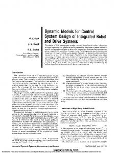
Numerical Examples: To verify the performance of the proposed model chosen the various sized examples of Safaei et al. [9] are solved by dynamic programming method with the C language by MATLAB/R2013a software on a Personal Laptop: Toshiba Satellite ProC650; Intel Mobile Core 2 Duo @ 2.10GHz processors and 2GB RAM and WINDOWS-7 operating system. To reduce the complexity, we relax decision variables yjp, y2jpmch, and z2jpch as continuous variables. It is worth noting that the minimization of the objective function and binary variable xjpmch in Eq. (3) insure that yjp is set to 0 or 1. In addition, binary

variables xjpmch, y1jpmch, and z1 jpch in Eqs. (12) 2 and (14) insure that decision variables y jpmch 2 and z jpch are also set to 0 or 1. The examples are generated according to the information provided in Table 1 inspired by the literature. In this table, term ‘‘U’’ implicates the uniform distribution. Σmajpm is equal to the number of alternative machines for processing operation j of part p. It is obvious that by increasing Σmajpm, the solution space increases progressively because the number of alternative process plans for each part operation increases.

Fig. 5: Flowchart of the Dynamic Programming Method. The datasets related to the first example are shown in Table 2. The first example consists of five part types, five machine types, and three periods where each part type is assumed to have three operations that must be processed, respectively. Each operation can be performed on two alternative machines. According to the complexity discussion above, there are about ([6 + 3]5)3 = 915 allocation combinations for the integrated model under the first example. The first four columns of Table 2 include the machine information, such as time capacity (hours), constant cost,

variable cost, and relocation cost. The demand quantity at each period, inter and intra-cell batch size, inventory and backorder costs, and the initial inventory for each part type are also shown in this table. By having linearized that, the proposed model consists of 1125 integer variables, 1578 non-integer variables, and 1383 constraints for the first example. For better observing the effect of the outsourcing on the cell configurations, the detailed optimal solution of the basis DCMS model (i.e., without considering the outsourcing) is shown in Table 3.


Page 24


Mohan and Rao

Table 1: Parameter Setting. Parameter Dph tjpm Σmajpm αm βm δm βpInter

Value U(100,1000) U(0,1) hour 2 j,p $ U(1000,2000) $ U(1,10) $ αm /2 U(10,50) units

βpIntra λp ηp ρp Iop

βpInter/5 $U(1,5) $U(1,5) $U(20,30) χ2(0,max{Dph})

Table 2: Typical Test Problem. Machine information α m β m δm Tm(h) $ $ $

P1 1

P2

2

3

500

1800

9

900

M1

500

1500

7

750

M2

500

1800

5

900

M3 0.73 0.93 0.44

500

1700

9

850

M4

500

1300

8

650

M5 0.54

Dph

1

2

P3 3

1

2

0.76 0.65 0.39 0.79

P4 3

2

3

1

2

0.33 0.57

0.74 0.40 0.63 0.45

0.59

0.14 0.93

0.26 0.48

0.67 0.62 0.12

0.75

Period1

300

800

200

0

250

Period2

400

700

700

200

0

Period3

400

0

450

950

350

35 7 5 5 30 0

25 5 4 4 29 0

20 4 5 5 20 300

40 8 4 4 26 150

45 9 3 4 24 0

Inter

βp Intra βp λp ηp ρp Iop

3

0.46 0.49 0.83 0.99

0.46 0.80 0.81

1

P5

γpinter = 50; γpintra = 5

Table 3: CASE-I (Optimal Solution for the basis DCMS Model). Optimal cost $100081.3

M/c Constant cost $34100

M/c Variable cost $62500

Intercell movement cost $754.2

Intracell movement cost $377.1

Reconfiguration cost $2350

Table 4: Optimal Production Plan for the First Example. P1 Qph Sph Iph Dph

300

300

H=1 P2 P3 1112 300* 438 600 261 100 850 200

P4 150*

P5 600

P1 435

150 0

350 250

35 400

P2

H=2 P3

P4

P5

50 200

350 0

P1 365

P2

400

0

H=3 P3 P4 1000

P5

450

350

450 700

700

950

Table 5: For Example-1 Comparison of Nima Safaei Vs P.N. Mohan.


Page 25


Optimal cost $100081.3 $113740

M/c Constant cost $34100 $36200

M/c Variable cost $62500 $66934

Inter-cell movement cost $754.2 $2719

Intra-cell movement cost $377.1 $4686

12.01

5.81

6.67

72.26

91.95

Reconfiguration cost $2350 $3200 26.56

P.N.Mohan N. Safaei Cost-Reduced (%)

Fig. 6: Optimal Cell Configurations for the First Example: (a) Period 1, (b) Period 2, and (c) Period 3.

Graph 1: For Example-1 Comparison of Nima Safaei (Series-1) Vs P.N.Mohan (Series-2). The cell configurations for three periods corresponding to the optimal solution of the DCMS model are shown in Figure 4, in which two cells are formed for each period. Part families, machine groups, part-operation allocation, and machine replication are also depicted in the cell configurations presented in Figure 6. For instance, three machines of type 1 are assigned to cell 1 in period 2. The cell is depicted as rectangular shape and the numbers within the cell represent the part-operations as numbered. For instance, operation 1 of part 1 in period 3 must be done by machine 5 in cell 1, operation 2 by machine 2 in cell 2, and operation 3 by machine 4 in cell 2, respectively. Thus, the processing part 1 in period 3 requires one inter-cell movement and

one intra-cell movement. One unit of machine 5 is added to cell 1 at the beginning of period 2. Also, one unit machine 1 is removed from cell 1 and 1 unit machine 3 is added to cell 2 at this time. CASE-II (Optimal solution for the basis DCMS Model) The second example consists of 10 part types, five machine types and four periods, in which each part type is assumed to have three operations that must be processed, respectively. Each operation can be performed on two alternative machines. Thus, there are more than (1010)4 combinations for allocating part operations to machines throughout the planning horizon. After linearization, the proposed model consists of 2940 integer


Page 26


Mohan and Rao

variables, 4078 non-integer variables, and 3566 constraints for the second example. The cell configurations corresponding to each period are depicted in Figure 7. As shown in this figure, no cell is formed in period 4 because of satisfying the demand by preceding periods. Also, as an example, the demand of part 1 at each given period is satisfied by subcontracting in the immediate previous period because of the existing lead time. As is

evident in the obtained results, which are with the Heuristic on software MATLAB/R2013a, it gives good accurate results when compared with examples of Safaei et al. [9] on Lingo software. From the obtained results plotted was shown in below, with which can say present developed model given the best optimal cost(s) compared to earlier safaei et al. [9].

Table 6: Best Obtained Solution for the Second Example. optimal cost $198722.6

M/c Constant cost $45800

M/c Variable cost $62500

InterCell movement cost $848.4

Intra-Cell movemen t cost $424.22

Reconfiguration inventory cost

Carryi ng cost

Backorder incurring cost

$8100

$49800

$13350

Table 7: Optimal Production Plan for the Second Example. h=1 P1 Qph Sph Iph Dph

P2 900+50*

P3 350

P4 88+150*

350

263 500

300 0

250 700

P5 202 154 599 800

P6 608+200*

P7

P8 550+100*

P9 350

P10 700

350

350 350

P1

P2

400 141 900

0

250 400

300

250 0

P3 782 18 631 150

h=2

P4 762

P5 845

250 250

400

h=3 P1 Qph Sph Iph Dph

P2

P3

400

600

800

400

250

650

P4

P5

0

P6 1422 120 630 650

P7 299

P8

P9 500

P10

300 0

250

500

350

P7 -

P8 -

P9 -

P10 -

h=4 P6

P7

P8 1000

P9 1500

300 0

750 250

900 600

300 250

Subcontr acting cost $17900

750

P10 472 228 30 450

P1 -

P2 -

P3 -

P4 -

P5 -

P6 -

Table 8: For Example-2 Comparison of Nima Safaei Vs P.N.Mohan. Optimal M/c M/c Inter-cell Intra-cell Reconfiguration Carrying Backorder Subcontracting cost constant variable movement movement Inventory cost cost incurring cost cost cost cost cost cost $198722.6 $399518 50.25

$45800 $46800 2.13

$62500 $80089 21.96

$848.4 $20079 95.77

$424.22 $2461 82.75

$8100 $17850 54.62

$49800 $68187 26.96

$13350 $15192 12.12

$17900 $148857 87.97

P.N.Mohan N.Safaei. Cost-reduced(%)

Fig. 7: Optimal Cell Configurations for the Second Example: (a) Period 1, (b) Period 2, and (c) Period 3.


Page 27


Graph 2: For Example-2 Comparison of Nima Safaei (Series-1) Vs P.N.Mohan (Series-2).

CONCLUSIONS In this paper, a novel mathematical and integrated model of the multi-period cell formation in a dynamic cellular manufacturing system (DCMS) has been introduced focusing on the operational aspects of the cell formation with the dynamic programming method and MATLAB/R2013a with C language software. This model is extended based on a basis DCMS model proposed in the literature (Safaei et al., 2009).Model given the best optimal cost. Most of the related studies use a multi-stage heuristic approach to first form the cells and then to plan production aspect of the manufacturing system and vice versa. However, the basis DCMS model is itself complex enough to be solved optimally in a reasonable time. Thus computational intelligent methods are proper alternatives to solve the proposed problem.

3.

4.

5.

6.

ACKNOWLEDGEMENTS We have great pleasure in expressing our deep sense of gratitude and sincere thanks to Prof. R. Tavakkoli-Moghaddam, Dr. Nima Safaei for their timely support while carrying out the work.

7.

REFERENCES 1. Wemmerlov U, Johnson DJ. Cellular manufacturing at 46 user plants: Implementation experiences and performance improvements. International Journal of Production Research. 1997; 35: 29–49p. 2. Rheault M, Drolet J, Abdulnour G.

8.


Physically reconfigurable virtual cells: A dynamic model for a highly dynamic environment. Computers and Industrial Engineering. 1995; 29(1–4): 221–5p. Kim B, Kim S. Extended model for a hybrid production planning approach. International Journal of Production Economics. 2001; 73: 165–73p. Wicks E-M, Reasor R-J. Designing cellular manufacturing systems with dynamic part populations. IIE Transactions. 1999; 31: 11–20p. Defersha F-M, Chen M. Machine cell formation using a mathematical model and a genetic algorithm based heuristic. International Journal of Production Research. 2006a; 44(12): 2421–44p. Safaei N, Tavakkoli-Moghaddam R, JabalAmeli S . A generalized cell formation problem in dynamic environment with different inter and intra-cell batch sizes. In: Dolgui A, Pereira C, Morel G (Eds). Information Control Problems in Manufacturing. Proceedings of the 12th IFAC International Symposium. Elsevier Science, Saint-Etienne, France. 17–19 May 2006; 2: 383–8p. Safaei N, Saidi-Mehrabad M, Jabal-Ameli MS. A hybrid simulated annealing for solving an extended model of dynamic cellular manufacturing system. European Journal of Operational Research. 2008; 185: 563–92p. Sankaran S, Kasilingam RG. On cell size and machine requirements planning in group technology systems. European Journal of Operational Research. 1993; 69: 373–83p.

Page 28


9. Safaei N, Tavakkoli-Moghaddam R. Integrated multi-period cell formation and subcontracting production planning in dynamic cellular manufacturing systems. Int. J. Production Economics. 2009; 120: 301–14p. 10. Harhalakis G, Nagi R, Proth J. An efficient heuristic in manufacturing cell formation for group technology applications. International Journal of Production Research. 1990; 28(1): 185– 98p. 11. Vakharia A, Kaku B. Redesigning a cellular manufacturing system to handle long-term demand changes: A methodology and investigation. Decision Sciences. 1993; 24 (5): 84–97p. 12. Balakrishnan J, Cheng C-H. Multi-period planning and un-certainty issues in cellular manufacturing: A review and future directions. European Journal of Operational Research. 2007; 177: 281–309p. 13. Chen M. A model for integrated production planning in cellular manufacturing systems. Integrated Manufacturing Systems. 2001; 12: 275–84p. 14. Olorunniwo F-O. Changes in production planning and control systems with implementation of cellular manufacturing. Production and Inventory Management. 1996; 37: 65–70p. 15. Benjaafar S, Sheikhzadeh M. Design of flexible plant layouts. IIE Transactions. 2000; 32: 309–22p. 16. Vakharia AJ, Moily JP, Huang Y. Evaluating virtual cells and multistage flow shops: An analytical approach. International Journal of Flexible Manufacturing Systems. 1999; 11: 291– 314p. 17. Venkatadri U, Rardin RL, Montreuil B. A design methodology for fractal layout organization. IIE Transactions. 1997; 29: 911–24p. 18. Askin RG, Ciarallo FW, Lundgren NH. An empirical evaluation of holonic and fractal layouts. International Journal of Production Research. 1999; 37(5): 961– 78p. 19. Chen M. A mathematical programming model for system reconfiguration in a dynamic cellular manufacturing

Mohan and Rao

20.

21.

22.

23.

24.

25.

26.

27.

28.

29.

30.


environment. Annals of Operations Research. 1998; 77: 109–28p. Heragu S-S, Chen J-S. Optimal solution of cellular manufacturing system design: Bender’s decomposition approach. European Journal of Operational Research. 1998; 107: 175–92p. Shang J-S, Tadikamalla P-R. Multicriteria design and control of a cellular manufacturing system through simulation and optimization. International Journal of Production Research. 1998; 3 6 : 1515–29p. Shinn A, Williams T. A stitch in time: a simulation of cellular manufacturing. Production and Inventory Management Journal. 1998; 39: 72–7p. Petrov V. Flow Line Group Production Planning. Business Publications, London; 1968. Hyer NL, Wemmerlo¨v, U. MRP/GT: A framework for production planning and control of cellular manufacturing. Decision Sciences. 1982; 13: 681–701p. Dale BG, Russell D. Production control systems for small group production. Omega. 1983; 11(2): 175–85p. Wemmerlov U. Production Planning and Control Procedures for Cellular Manufacturing. American Production and Inventory Control Society, Falls Church; 1988. Askin RG, Mitwasi MG. Integrating facility layout with process selection and capacity planning. European Journal of Operational Research. 1992; 57: 162–73p. Habich M. Koordination autonomer Fertigungsinseln durch ein adaptiertes PPSKonzept. Zeitschrift fu¨r wirtschaftliche Fertigung. 1989; 84(2): 74–7p. Rohloff M. Decentralized production planning and design of a production management system based on an objectoriented architecture. International Journal of Production Economics. 1993; 30–1p, 365–83p. Banerjee SK. Methodology for integrated manufacturing planning and control systems design, 54–88. In: Artiba A, Elmaghraby SE. (Eds). The Planning and Scheduling of Production Systems, Methodologies and Applications. Chapman & Hall, London; 1997.

Page 29


31. Schaller J-E, Selc-uk Erengu¨c-, S, Vakharia A-J. A methodology for integrating cell formation and production planning in cellular manufacturing. Annals of Operations Research. 1998; 77: 1–21p. 32. Chen M, Cao D. Coordinating production planning in cellular manufacturing environment using tabu search. Computers & Industrial Engineering. 2004; 46: 571–88p. 33. Defersha FM, Chen M. A comprehensive mathematical model for the design of cellular manufacturing systems. International Journal of Production Economics. 2006b; 103: 767–83p. 34. Nomden G, Van der Zee D-J. Virtual cellular manufacturing: configuring routing flexibility. International Journal of Production Economics. 2008; 112: 439–51p. 35. Ioannou G. Time-phased creation of

hybrid manufacturing systems. International Journal of Production Economics. 2006; 102: 183–98p. 36. Kioon S-A, Bulgak A-A, Bektas T. Integrated cellular manufacturing systems design with production planning and dynamic system reconfiguration. European Journal of Operational Research. 2009; 192: 414–28p. 37. Mungwattana A. Design of Cellular Manufacturing Systems for Dynamic and Uncertain Production Requirements with the Presence of Routing Flexibility. PhD Thesis. Submitted to the Faculty of the Virginia Polytechnic Institute and State University, Blackburg, VA. 2000. 38. Tavakkoli-Moghaddam R, Aryanezhad MB, Safaei N, et al. solving a dynamic cell formation problem using metaheuristics. Applied Mathematics and Computation. 2005; 170(2): 761–80p.


Page 30