Jan 2, 2005 - which is characterized after a study of the simulation data. We also validate the proposed solutions by using a physical model and properties of ...
Dynamic Classification of Defect Structures in Molecular Dynamics Simulation Data S. Mehta∗
S. Barr†
T. Choy†
H. Yang∗
S. Parthasarathy∗
R. Machiraju∗
J. Wilkins† Department of Computer Science and Engineering, Ohio State University † Department of Physics, Ohio State University Contact: {mehtas,srini,raghu}@cse.ohio-state.edu
∗
January 2, 2005 Abstract In this application paper we explore techniques to classify anomalous structures (defects) in data generated from abinitio Molecular Dynamics (MD) simulations of Silicon (Si) atom systems. These systems are studied to understand the processes behind the formation of various defects as they have a profound impact on the electrical and mechanical properties of Silicon. In our prior work we presented techniques for defect detection [11, 12, 14]. Here, we present a two-step dynamic classifier to classify the defects. The first step uses up to third-order shape moments to provide a smaller set of candidate defect classes. The second step assigns the correct class to the defect structure by considering the actual spatial positions of the individual atoms. The dynamic classifier is robust and scalable in the size of the atom systems. Each phase is immune to noise, which is characterized after a study of the simulation data. We also validate the proposed solutions by using a physical model and properties of lattices. We demonstrate the efficacy and correctness of our approach on several large datasets. Our approach is able to recognize previously seen defects and also identify new defects in real time. 1 Introduction Traditionally, the focus in the computational sciences has been on developing algorithms, implementations, and enabling tools to facilitate large scale realistic simulations of physical processes and phenomenon. However, as simulations become more detailed and realistic, and implementations more efficient, scientists are finding that analyzing the data produced by these simulations is a non-trivial task. Dataset size, providing reasonable response time, and modeling the underlying scientific phenomenon during the analysis are some of the critical challenges that need to be addressed.
In this paper we present a framework that addresses these challenges for mining datasets produced by Molecular Dynamics (MD) simulations to study the evolution of defect structures in materials. As component size decreases, a defect - any deviation from the perfectly ordered crystal lattice in a semiconductor assumes ever greater significance. These defects are often created by introducing extra atom(s) in the Silicon lattice during ion implantation for device fabrication. Such defects can aggregate to form larger extended defects, which can significantly affect device performance in an undesirable fashion. Simulating defect dynamics can potentially help scientists understand how defects evolve over time and how aggregated/extended defects are formed. Some of these defects are stable over a period of time while other are short-lived. Efficient, automated or semi-automated analysis techniques can help simplify the task of wading through a pool of data and help quickly identify important rules governing defect evolution, interactions and aggregation. The key challenges are: i) to detect defects; ii) to characterize and classify both new and previously seen defects accurately; iii) to capture the evolution and transitioning behavior of defects; and iv) to identify the rules that govern defect interactions and aggregation. Manual analysis of these simulations is a very cumbersome process. It takes a domain expert more than eight hours to manually analyze a very small simulation of 8000 time frames. Therefore, a systemic challenge is to develop an automated, scalable and incremental algorithmic framework so that the proposed techniques can support in-vivo analysis in real time. In our previous work [11, 12, 14], we presented algorithms to address the first challenge. Here we address the second challenge coupled with the systemic challenge outlined above. The design tenets include not only accuracy and execution time but also both statistical and physical validation of the proposed models. We also present preliminary results
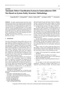
to show that our approach can aid in handling the third challenge. The main contributions of our application case study paper are: 1. We develop a two-step incremental classifier that classifies both existing and new defects (generates a new class label). 2. We validate each step of our 2-step classifier theoretically, relying on both physical and statistical models. 3. We validate our approach on large (greater than 4GB) real MD simulation datasets and demonstrate both the exceptional accuracy and efficiency of the proposed framework. 4. We present initial results which show that our approach can be used to capture defect evolution and to generate labeled defect trajectories. Our paper is structured in the following manner. Section 2 discusses the basic terminology of MD and related work. An overview of our framework is provided in Section 3. We present our algorithm in Section 4. Results on large simulation datasets are presented in Section 5. Finally, we conclude and discuss directions for future work in Section 6. 2 Background and Related Work 2.1 Background: In this section, we first define basic terms that are used throughout this article. Later, we describe pertinent related work. A lattice is an arrangement of points or particles or objects in a regular periodic pattern in three dimensions. The elemental structure that is replicated in a lattice is known as a unit cell. Now, consider adding a single atom to the lattice. This extra atom disturbs the geometric structure of lattice. This disturbance, comprised of atoms which deviate from the regular geometry of lattice is referred to as the defect structure. Defects created by adding an extra atom are known as single-interstitial defects. Similarly one can define di- and tri-interstitial defects by adding two or three single interstitial defects in a lattice respectively. Figure 1(a) shows a Si bulk lattice with a certain unit cell shaded differently (black). Figure 1(b) shows another lattice with a single interstitial defect. Figure 1(c) depicts two interstitials: in the lower left and upper right corners respectively of a 512-atom lattice. The different shades again represent separate and distinct defects. We use the Object-Oriented High Performance Multiscale Materials Simulator (OHMMS) that some of us developed (primarily led by co-author Wilkins) [4] as our workhorse. The equation of motion as described by Newton’s second law is used to determine atom locations. While the exact forces must be derived from quantum mechanical
studies and computations, these classical equations serve as a suitable approximation. 2.2 Related Work: Traditionally, physicists have used ground energy and electrostatic potential to find defects in lattice. For example ab-initio methods are used to locate interstitial defects in a Si lattice [2, 19]. These methods exploit anomalies in the energy/potential fields available at all points in the lattice . However, the calculation and analysis of these energies/potential is very time consuming. The most pertinent work that is closely related to our own work employs the method of Common Neighbor Analysis (CNA) [3, 8]. CNA attempts to glean crystallization structure in lattices and uses the number of neighbors of each atom to determine the structure sought. However, it should be noted that the distribution of neighbors alone cannot characterize the defects, especially at high temperatures. Related to our work is the large body of work in biomolecular structure analysis [1, 10, 16, 20]. In these techniques, the data is often abstracted as graphs and transactions and subsequently mined. However, such an abstraction often does not exploit and explain many of the inherent spatial and dynamical properties of data that we are interested in. Moreover, while some of these techniques [17, 20], deal with noise in the data, the noise handling capabilities are limited to smoothing out uncorrelated and small changes in spatial location of atoms. Within the context of MD data, noise can also change the number of defect atoms detected, for essentially the same defect structure at different time frames. None of the methods in the biological data mining literature deal with this uncertainty. Matching of two structures has drawn a lot of attention in recent past. Zhang et al.[22], propose a protein matching algorithm that is rotation and translation invariant. This method relies on the shape of the point cloud and it works well for proteins given the relatively large number of atoms; the presence of a few extra atoms does not change the shape of point cloud. A potential match is not stymied by the presence of extra atoms. However, in MD simulation data, we are interested in anomalous structures which can be as small as just six atoms. Extra atoms that may be included in a defect given the thermal noise will skew a match significantly even if the two defects differ by one atom. Geometric hashing, an approach that was originally developed in the robotics and vision communities [21], has found favor in the biomolecular structure analysis community [15, 20]. Rotation and translations are well handled in this approach. The main drawback of geometric hashing is that it is very expensive because an exhaustive search for optimal basis vector is required. A more detailed discussion on various shape matching algorithms can be found in the survey paper by Veltamp and Hagedoorn [18]. We use statistical moments to represent the shape of a defect for initial pruning. The seminal work by Hu [13] described a set of seven moments which
Figure 1: (a)Original lattice with unit cell marked (b)Lattice with one interstitial defect (c)Lattice with two interstitial defects
captures many of the features of a two-dimensional binary images. In recent work, Galvez [7] proposed an algorithm which uses shape moments to characterize 3D structures using moments of its two-dimensional contours. However, owing to relatively small number of atoms present in a typical defect, the contours or the corresponding implicit 3D surface are impossible to obtain with accuracy. 3
Dynamic Classification Framework
Figure 2 shows our framework for MD simulation data analysis. The framework is divided into 3 phases. Phase 1 Defection Detection: this phase detects, spatially clusters (or segments) defects and handles periodic boundary conditions. Detailed explanation on this phase is given in our earlier work [11, 14, 12]. Phase 2 - Dynamic Classification: this phase classifies each defect found in Phase 1. This phase consists of three major components: 1. Generating a feature vector for each detected defect. This feature vector is composed of weighted statistical moments. 2. Pruning the defect classes based on the feature vector. This step provides a smaller subset of defect classes to which an unlabeled defect can potentially belong to. 3. An exact matching algorithm that assigns the correct class label to the defect. This steps takes into account the spatial position of the atoms. The defect is assigned a class label if it matches with any of the previously seen defects, otherwise the defect is considered new. Phase 2 maintains 3 databases for all detected defects. Section 4 gives detailed information regarding these three databases and their update strategies. The framework is made robust by modeling noise in both Phase 1 and Phase 2. Our noise characterization models the aggregate movement of the defect structure and the arrangement of the atoms (in terms of neighboring bonds). Our framework can be deployed to operate in a streaming fashion. This is important since it enables us to naturally handle data in a continuous fashion while a simulation is in
progress. Phase 1 handles the entire frame and detects all the defects. Each defect is then pipelined into Phase 2. Thus, we are able to incrementally detect and classify defects while consistently updating the database in real time. Phase 3 - Knowledge Mining: this phase uses the databases generated by Phase 2. These databases store the information about all the defects in a given simulation. These databases can be used to track and generate the trajectories of the defects, which can assist us to better understand the defect evolution process. Additionally, various data mining algorithms can be applied on the databases. Mining spatial patterns within one simulation can aid in understanding the interactions among defects. Finding frequent patterns across multiple simulations can help to predict defect evolution. In this paper, we describe Phase 2 in detail. We also show some initial results for Phase3. 4 Algorithm Our previous work [11, 12, 14] describes the defect detection phase in detail. Every atom in the lattice is labeled either as a bulk atom or as a defect atom. However, upon further evaluation we found that this binary labeling is not well suited for robust classification of defect structures. Therefore, we propose to divide the atoms into three classes based on their membership or proximity to a defect. We also validate the correctness of this taxonomy by using a physical model. Our taxonomy is: • Core-Bulk Atoms (CB): The atoms which conform to the set of rules defined by the unit cell are bulk or non-defect atoms. Bulk atoms which are connected exclusively to other bulk atoms are labeled as core bulk atoms. • Core-Defect Atoms (CD): The atoms which do not conform to the set of rules are defect atoms. All the defect atoms which are connected to more defect atoms than bulk atoms are labeled as core defect atoms. These
&'
()
!
"
& &
#
$
%
!
Figure 2: Defect Detection and Classification Framework
atoms dominate the shape and properties of a defect. • Interface Atoms (I): These atoms form the boundary between a core bulk atom and a core defect atom. These atoms fail to conform to the prescribed set of rules by a small marginally (i.e. the thresholds for bond lengths and angles, are violated in a marginal way) thus are marked as defect atoms; however, the majority of their nearest neighbors are core bulk. Thus, they form a ring between core bulk atoms and core defect atoms. Presence or absence of these atoms can considerably change the shape of a defect, which makes matching of defect structures very difficult.
(a)
(b) )
Figure 3: (a) Original Defect (b) Detected Defect with extra atoms
Figure 4(a) illustrates all three types of atoms. The black atoms belong to core defect, white atoms form core bulk and the gray atoms are interface atoms. We next, justify this an atom while solving MD equations. The physics behind taxonomy. springs can be used to calculate these energies. Hooke’s law for springs states that the force exerted by a spring is proPhysical Validation: A lattice system can be represented portional to the distance by which it is stretched. The energy by the Mechanical Molecular Model as follows: atoms are of a spring can be derived by using relationship between enrepresented by spheres, and bonds by springs connecting ergy and force. The energy is calculated by the following these spheres. The energy of an atom in the lattice system equation: is calculated by the following equation: 1 Etotal = Elength + Eangle + Einteractions E = Kδ 2 (4.1) 2 where Elength and Eangle are the energies due to bond where K is the spring constant and δ is the distance by which stretching and angle bending respectively. Also, each atom a spring is stretched from its uncompressed state. in the lattice interacts with every other atom. Einteractions Elength and Eangle for each atom can be computed by usaccounts for energy generated by these interactions. How- ing appropriate spring constants, Klength and Kangle reever, we can ignore Einteractions for the MD datasets be- spectively. Information about the ideal bond length and cause OHHMS only considers the effect of first neighbors of bond angle present in the existing literature can be used
for uncompressed spring state. Drexer [5] lists the values for Klength and Kangle as 185 N ewton/meter and 0.35 N ewton/radian respectively for the Silicon lattice. For each atom we find the bond lengths and bond angles it forms with its first neighbors and then find the δs. Core bulk atoms deviate very little from the ideal bond angle and bond length, therefore their corresponding δs should be very low; whereas for core defect atoms the δs should be high. Since the energy is directly proportional to δ 2 , core bulk atoms should have low energy whereas core defect atoms should have high energy. To validate our taxonomy, we sampled 1400 frames from different simulations and calculated the energy for each atom in the lattice. Figure 4(b) shows the distribution of energy. It is clear from the distribution that the majority of the atoms have very low energy (∈ [0, 0.2]). These atoms are core bulk atoms. The core defect atoms have very high energy (≥ 1.2). All the atoms which lie between low and high energy levels are interface atoms. Thus, this physical model clearly validates our taxonomy of atoms. Therefore we refine our original binary labeling [11] of individual atoms by further dividing defect atoms into core defect atoms and interface atoms. Before describing the classification method, we discuss the challenges which need to be addressed to build a robust and efficient classifier for MD data. We list each of them and describe how they are addressed within the context of the proposed algorithm. For each proposed solution we also provide the physical validation using the Mechanical Molecular Model and properties of the lattice system. 4.1
Challenges and Proposed Solutions
4.1.1 Thermal Noise: Thermal agitations can cause atoms to change their spatial positions. Such changes can potentially have two kinds of effect on the defect structures:
number of its neighbors. To model this behavior we define a random variable Di : Di =
1 F +1 (Mi
+
F P j=1
Mj )
where Mi is the displacement of atom i between two consecutive time steps, having F first neighbors within a distance ˚ (bond length for Si), and i ∈ [1, N ], N being the of 2.6A total number of atoms in the lattice. We empirically observe that Di can be effectively approximated by using a normal distribution with parameters, µnoise and σnoise (the average mean and standard deviation of all Di s). We found µnoise to be very close to 0 (which is expected because a given atom cannot move very far from its original location between two consecutive time frames). The parameter σnoise is used to model the effect of noise in the defect classification algorithm. From a set of randomly selected 4500 frames, we ˚ found the value of σnoise to be 0.19A. Physical Validation: The noise threshold can be validated by using the Mechanical Molecular Model. The bond energy B of Si-Si bond is 52 Kcal/mol, which is the amount of energy needed to break a Si-Si bond. Using Equation 4.1 we can compute the maximum distance a Si atom can be displaced before the bond is broken. Essentially we solve the following equation for the value of δ : B ≤ 12 Kδ 2 By substituting the values of K and B we found the value ˚ which implies that two bonded atoms cannot of δ to be 0.2A ˚ apart without breaking the bond be moved more than 0.2A between them. Thus, the empirically observed value is very close to the theoretical value given by the physical model.
To solve the second problem posed by thermal noise, we propose a weighting mechanism. The weighting mechanism 1. The precise location of the atoms and their inter-pair is based on the following two observations: • Observation 1: In two consecutive time frames the core distances will not be exactly the same from frame defect atoms cannot change considerably. to frame. Thus the classification method should be tolerant to small deviations in the spatial positions. • Observation 2: Interface atoms can make a transition from bulk to defect (and vice-versa) very quickly. 2. The change in the spatial positions can also force a previously labeled bulk atom to violate the rules and Figure 3(a) and Figure 3(b) show the defect detected from be labeled as a defect atom (and vice versa) in the next two different frames after applying local operators. The time frame. Therefore the number of atoms in a defect defect in Figure 3(b) has extra atoms (interface) but the can change, which in turn changes the overall shape of core defect (black atoms) remains unchanged. Therefore, the defect structure which makes the classification task a weighting mechanism is proposed to reduce the influence of interface atoms relative to that of core atoms within a more difficult. defect structure. Essentially, the weight assigned to each To address the first problem we consider a data driven atom in a given defect is proportional to the number of its approach to derive noise thresholds. From our study of first neighbors in the defect structure. Thus core defect physics, we know that the change in position of each atom atoms contribute more to defect classification than interface in two consectutive frames is influenced by the position and atoms. These weights are also used for handling translations
(a)
(b)
Figure 4: (a) Taxonomy of atoms (b) Energy Plot
(described below) and for computing the feature vector moments capture skewness in defects. To account for the (weighted moments). interface atoms we calculate weighted moments instead of simple moments. (Recall that the weighting mechanism Physical Validation: Observation 1 can be explained as assigns high weights to core defect atoms and low weights to follows. Each atom in the lattice interacts most with its first interface atoms). The feature vector comprising of weighted neighbors. The greater the number of first neighbors of an moments of a defect is calculated as : atom, the more connected it is and hence the more restricted N P its movement. The core defect atoms have high connectivity p 1 m n Wmnp = P wi ∗ Dix ∗ Diy ∗ Diz N with other defect atoms, which makes it more difficult for wj i=1 them to move very far in a short period of time. j=1 Observation 2 can be explained as follows. Interface atoms where m + n + p ≤ 3 labeled as defect (or bulk), usually fail (or conform to) the set of rules by a small margin. A very small variation in their th spatial locations can change their labels. These interface where Dix is the x-ordinate of i atom of defect D. An imatoms, however, are very loosely connected to the core defect portant property of this feature vector is that it is translation invariant if the weighted center of mass (given by the first atoms. Most of their first neighbors are core bulk atoms. To summarize, over a period of time core defect atoms will three weighted moments) is translated to zero. change considerably less than interface atoms. Therefore Since all the rotations in the lattice are symmetry operations more emphasis (weight) should be given to core defect atoms (see below for an explanation of symmetry operation), rotawhile matching two defect structures. This is precisely what tional ambiguity can be resolved easily by applying the appropriate permutation on the feature vector. For example, if our weighting mechanism does. the defect is rotated by 180 degrees across the X-plane (a 4.1.2 Translational and Rotational Invariance: Transla- mirror transform), all the moments involving an odd power tions and rotations pose another problem in defect classi- of the X-component will change sign. In a similar fashion, fication. The same defect can occur in different positions all the rotations can be resolved by checking the pre-defined and orientations in the lattice. To classify a defect correctly, permutations of original moments. There are a total of 3 firsttranslations and rotations should be resolved before assign- order moments, 6 second-order moments and 10 third-order ing the class. We next present our approach to attain transla- moments. Of these, since the center of mass is translated to the origin (to deal with translations), W100 , W010 and W001 tional and rotational invariance. are all zero. Therefore we have a 16-dimensional feature Feature Vector Generation: We describe the shape of vector represented by Dw . a defect by using statistical moments. We chose to use all first, second and third order moments. Third order Physical Validation: Interface atoms change the shape of the defect, which can change the center of mass considerably.
Therefore using center of mass without the weights can assign a new class label to a defect even if the core defect is not new. Thus core defect atoms should contribute more towards the calculation of the center of mass. A lattice cannot be rotated in arbitrary directions. The only rotations possible in the lattice are those which carry the lattice onto itself. This means that after rotation each atom of the lattice is exactly at a position occupied by an atom prior to the rotation. These rotations are known as symmetry operations [9]. Under this constraint, only a finite number of rotations are possible in lattices. For example, in the Si lattice system only 24 types of rotations are possible.
namic [6]. The classifier should be dynamic in the classical sense, as in new streaming data elements can be classified, but should also be dynamic in the sense that new classes(defects) if discovered can be added to the classifier model in real time. The new defect should be available when the next frame is processed. We next present our two-step classification process which integrates all the proposed solutions to the above-mentioned challenges.
4.2 Two Step Classification Algorithm: P hase1 of our framework detects the defect(s) from the lattice as mentioned in Section 3 P hase2 classifies the defect(s) de4.1.3 Shape Based Classification: While matching two tected in P hase1. Given a defect D, the goal is to find the defect structures, the classifier should take into account the type T of this defect. If D does not match any of the prepositions of all individual atoms in the defects. This atom-to- viously seen defects in the simulation, it is labeled as a new atom matching is relatively expensive. Furthermore because defect and stored in the databases IDshape and IDmoment , of large number of defect classes present in simulation where ID is a unique simulation identification number, datasets, it would be unrealistic to carry out such an atom- IDshape stores the actual three dimensional co-ordinates and to-atom matching for all classes at each and every time IDmoment stores the weighted central moments (feature vecstep. Therefore a scheme is needed to effectively reduce the tor) of the defect structure. These databases store all the number of candidate classes on which an exhaustive atom- unique defects detected in the current simulation. The label to-atom matching is performed. of a new defect is of the form defect i j, indicating that the We address this challenge by adopting a two step classifi- new defect is the j th defect in the ith frame of the simulacation process. The first step uses weighted moments to tion. If D is not new then a pointer to the defect class which find a smaller subset of defect classes to which the unla- closely matches D is stored. Besides these two databases beled defect can potentially belong and passes it to the next a summary file is generated which stores names of all destep. Weighted moments (feature vector) are used because tected defects in the simulation along with corresponding moments are known to capture the overall shape of an ob- frame numbers. We now proceed to describe the two steps ject [13]. The second step then finds the closest class by of our classifier in detail. taking into account the positions of the atoms and their arrangement in three dimensional space. In essence, both 4.2.1 Step 1 - Feature Vector based Pruning: We use steps use the information about the shape of a defect. The a variant of the KNN classifier for this task. The value of first step uses the high level information about defect struc- K is not fixed: instead, it is determined dynamically for ture whereas the next step refines it by matching individual each defect. Given the feature vector (DW ) of a defect atoms. We achieve the desired efficiency because the first D, we compute and sort the distances between DW and step is computationally very cheap and reduces the search IDMi , where IDMi is the mean moment vector of the ith space considerably for the next step. Experimental results to defect in IDmoment . All classes having distances less than corroborate this are shown in Section 5. an empirically-derived threshold are chosen as candidate classes. Step 2, then, works on these K classes only. If Physical Validation: The majority of the physical properties no class can be selected, D is considered as a new defect. of a defect are governed by its shape. Most of the stable Databases ID shape and IDmoment are updated immediately, defects seen so far have a very compact shape. Unstable so that D is available when the next frame is processed. structures tend to re-organize the atoms to form such a In a similar fashion, one can use Naive Bayes and Voting compact structure. The movement of the defect in the lattice based classifiers. Like the KNN classifier, these classifiers is also governed by the shape of the defect. also provide metrics which can be used to select the top K candidate classes. More specifically, a Naive Bayes classifier 4.1.4 Emergence of new defect classes: The underlying provides the probabilities of a feature vector belonging to motivation of our effort is to discover information which can each class, and a voting based classifier gives the number of assist scientists to better understand the physics behind de- votes for each class. The top K classes can then be chosen fect evolution, ideally in real time. This defect evolution based on probabilities and votes. We chose VFI as our voting can result in new defect classes which are not in existing based classifier. As for other types of classifiers, such as the literature. This requires the classification process to be dy- decision tree-based ones, it is not trivial to pick K candidate
classes, therefore they are not considered in this work. From the three applicable classifiers, the KNN classifier is chosen because it gives the highest classification accuracy, as described in Section 5. Besides its high accuracy, the KNN classifier is incremental in nature. In other words, there is no need to re-build the classification model from scratch if a new class is discovered. In contrast, Naive Bayes and VFI will require the classification model to be re-built every time a new class is discovered. The K candidate classes are passed to Step 2. The representative shapes of these K classes are matched using an exact shape matching algorithm based on the Largest Common Substructure (LCS). Next, we explain the main steps of our exact matching approach. 4.2.2 Step 2 - Largest Common Substructure based algorithm: Assume, A is a defect of unknown type and B is the median defect representing one of the candidate classes from Step 1. The defects are mean centered and the rotation is resolved. We next describe all the steps of the LCS algorithm in detail. • Atom Pairs Formation: The defects are sorted w.r.t. their x-ordinate. Two atoms i and j in defect A form an atom pair Aij if distance(Ai ,Aj ) ≤ bond length. This step uses the information about neighbors and connectivity calculated in Phase 1. These atom pairs are calculated for both defects. For each atom pair Aij , we store the projection onto X,Y and the Z-axes represented by Aijx , Aijy and Aijz respectively. • Find matching Pairs: For each pair Aij we find all pairs Bkl such that |Aijx − Bklx | ≤ σnoise |Aijy − Bkly | ≤ σnoise |Aijz − Bklz | ≤ σnoise where threshold σnoise is obtained as explained in Section 4.1.1.
Before explaining each step in detail, we define the notion of compatible substructures: Two substructures U and V are considered compatible w.r.t. the rule Aij ↔ Bkl , if the last atom added to U is the ith atom of defect A and the last atom added to V is the k th atom of defect B. Being compatible implies that the two substructures have the same number of atoms and the orientation of atoms (which defines shape) is approximately same (within noise thresholds). The algorithm starts by finding all compatible substructures U and V w.r.t to the rule Aij ↔ Bkl (Line 4). The length of U (and V ) is increased by 1 and atom j (and l) is added. Lines 5-10 of Figure 5 show this process. However, if no compatible substructures are found then a new substructure U (and V ) is initialized with atoms i and j (k and l). Lines 11-16 in Figure 5 refer to this case. The same process is then repeated for all the rules. 1 Input : All rules 2 For each rule : Aij ↔ Bkl 3 { 4 Find Compatible substructures U and V 5 If U and V found 6 { 7 Length = Length+1; 8 U [Length] = j; 9 V [Length] = l; 10 } 11 else 12 { 13 Create new U and V ; 14 Store i and j in U ; 15 Store k and l in V ; 16 } 17 }
We represent this equality of atom pairs as Aij ↔ Bkl , Figure 5: Pseudo code for finding Largest Common Subwhich implies that the length and orientation of the structure bond formed by atoms i and j of defect A is similar This method also provides the correspondence between to the bond formed by atoms k and l of defect B. atoms. Atoms in U and V have a one-to-one relationBy comparing each projection separately, we intrinsiship between them. cally take care of both: bond length and orientation. • Similarity Metric Computation: The Largest • Find Largest Common Substructure (LCS): The Structure (LS) is then chosen from the common subrules generated in the previous step are used to find the structures. We use the following metric to determine largest common substructure between two defects. We the similarity between A and B: use a region growing based approach to find LCS. The pseudo code for finding LCS is shown in Figure 5.
Sim(A, B) =
2 ∗ kLSk kAk + kBk
100 90 80 70
Accuracy(%)
This similarity is calculated between A and all the K candidate defect classes. The class which gives the maximum similarity greater than a user defined threshold is chosen as the target class. If the maximum similarity is less than the user defined threshold the defect is considered new and both the databases, IDshape and IDmoment are updated. The summary database is updated for each defect (previously seen or new).
60
Unweighted Moments Weighted Moments
50 40 30 20
5 Experiments and Results In this section we present the results of our framework. As noted earlier we use OHMMS (see Section2) to generate the datasets. We first, show the advantage of weighted moments over unweighted moments by comparing the accuracies of various classifiers. Next, we demonstrate the accuracy of the LCS algorithm bootstrapped with different classifiers: KNN, Naive Bayes and VFI. Later, we show the scalable aspects of our framework by deploying it on very large datasets (in the giga-byte range). Finally, we present preliminary results demonstrating how our two-step classifier can help us gain a better understanding of defect evolution.
10
Jr ip
(K =1 ) KN N
SM O
on eR
VF I D ec is io nt re e
LW L H yp er pi pe
N aï ve
Ba ye s
0
Classifier
Figure 6: Accuracies of various classifiers
An important point to note is that all the 1, 400 defects used for this experiment were labeled manually by a domain expert. However, in actual simulation data there are no predetermined labels since new classes can be created as the simulation progresses. Also there is no training data to build the initial model for Decision tree and Naive Bayes 5.1 Robust Classification: To illustrate the importance of classifiers. For the purpose of this experiment, we artificially using weighted moments as opposed to unweighted mo- divided the dataset into training (90%) and testing data ments, we performed the following experiment: a total of (10%) for all the classifiers that require training data to build 1, 400 defects were randomly sampled across multiple simu- model. Classifier accuracies are averaged over 10 runs of the lations conducted at different temperatures. The noise in the classifiers. simulation depends on the temperature at which the lattice is Only KNN and VFI can discover new classes in real time. simulated. Therefore two defects belonging to the same class Both classifiers calculate a similarity metric for classificacan have different number of atoms and/or different positions tion: distance in the case of KNN and votes for VFI. If this of atoms depending on the temperature, even though their similarity metric is less than a user defined threshold, a new core defect shape remains approximately the same. This class label can be assigned to the defect. However, VFI will sampling strategy ensures that no two defects of the same have to build the whole classification model from start whenclass are exactly the same. Each defect, in this experiment, ever a new defect class is discovered. Since large number of belongs to one of the fourteen classes of single interstitial defect classes can be created in a simulation, rebuilding the defects that are known to arise in Si. classification model repeatedly will degrade the performance For comparison purposes, we tried nine different classifiers. considerably. Figure 6 clearly demonstrates that all classifiers perform better when weighted moments were used. Classification accuracies of VF1, KNN (K=1) and Decision tree based classifiers are comparable (close to 90%). SMO (SVM based classifier), also provided good accuracy (85%) but it was quite slow; classifying 1,400 defects took over 25 minutes. On average the classification accuracy increased by 8% when weighted moments were used. Unweighted Moments Next, we present the classification accuracies of Naive Weighted Moments Bayes, KNN and VFI. These classifiers are modified to pick the K most important classes dynamically (as explained in Section 4). Figure 7 shows the results for this experiment. KNN with weighted moments outperforms all other classifiers by achieving an accuracy of 99% whereas Naive Classifier Bayes is the least accurate with an accuracy of 86%. Again, weighted moments outperform unweighted moments. Figure 7: Classification accuracy with Dynamic K 100
90 80
Accuracy(%)
70 60 50 40 30 20 10
0
KNN
Bayes
VfI
(a)
(b)
(c)
Figure 8: Transitions in Three Interstitials(a) 1st Frame (b) 20000th frame (c) 130,000th frame
Thus the LCS algorithm bootstrapped with the KNN classifier using weighted central moments is the best choice in terms of accuracy and efficiency.
as defect atoms (and vice versa). As a result, there exist marginal fluctuations in the shape of a defect from frame to frame. However, the effect of these changes on weighted central moments is relatively small. For example, in the 5.2 Scalable Classification - Large Simulations: We use Three Interstitials dataset, the total number of defect instanthree large datasets, namely Two Interstitials, Three Inter- tiations in the simulation was around 320, 000. However, our stitials, and Four Interstitials for these experiments. Ta- classifier detected only 1, 543 unique defect classes. These ble 1 summarizes the number of frames, size of the dataset, 1, 543 defects capture the actual transitions as verified by a total number of defects present in the simulation and number domain expert. To reiterate, the use of weighted moments of unique defect classes identified by our framework. For all minimizes false positives and ensures robust classification. three datasets, our framework was able to correctly identify The use of weighted moments and pruning in Step 1 also all the defect structures. However, given the paucity of space allows our approach to achieve good scalability. Finding we only present an in-depth analysis of the Three Intersti- the LCS is a relatively expensive algorithm, therefore we tials dataset. Similar results were also obtained for other want to use it as infrequently as possible. In most cases the datasets. number of candidate classes K from Step 1 (KNN classifier) of our dynamic classifier is less than 3. For example, in Dataset Number of Size Total Defects Unique Defects the Two interstitials dataset 2, 841 unique defects were Frames (in GB) Detected found however, the LCS algorithm only evaluates less than Two Interstitials 512,000 4 350,000 2,841 3 closest matches. This underlines the usefulness of the Three Interstitials 200,200 6 320,000 1,543 pruning step of our classifier. The discovery of all the Four Interstitials 297,000 10 410,000 3,261 unique defect classes demonstrates that the correct defect class is not pruned away. To summarize, pruning based Table 1: Datasets Used in Evaluation on weighted moments provides scalability to the framework without affecting the accuracy. Many of these defects are not stable, i.e, they may exist This simulation starts with three disconnected interstitial for as few as 100 time frames; however these unstable defects. The defects move around in the lattice during the defect structures are extremely important since they allow th first 19, 000 time frames. However, at the 20, 000 time one to understand the physics behind the creation of, and frame two of the defects join and form a ’new’ larger defect. transitioning to, stable structures. We can easily eliminate This larger defect does not change for a long period of these unstable structures from our repositories by either th time. However, at the 130,000 time frame the third defect maintaining simple counts or by time averaging the frames. joins the ’new’ defect and forms a single large defect which However, using both these techniques will result in loss of remains unchanged until the end of the simulation. Figure 8 transition information. To illustrate this point we took the shows the evolution of the defects in the simulation. For the same Three Interstitials dataset and averaged it over every rest of this paper we refer to changes in defect shape or type 128 frames. In this averaged data, we found only 18 unique as ”transitions”. defects. It turns out that we found all the possible stable Though these transitions occur over a large period (thoustructures, but the actual transitioning behavior was lost. sands of time steps), atoms do not stay at the exact same position in two consecutive frames due to thermal noise. Such thermal agitations can also cause bulk atoms to be labeled
5.2.1 Timing Results: Figure 9 shows the time taken by OHHMS to complete the simulation and time taken by our framework to analyze the data. The figure also shows the individual time taken by Phase1 (defect detection) and Phase2 (classification). Phase1 takes around 45% of the time and Phase2 requires the rest of the time. All the experiments are carried out on Pentium 4 2.8GHz dual processor machine with 1 GB of main memory. Our classifier can analyze the data almost 1.5 times faster than the data generation rate. This allows us to analyze the data and build the defect databases in real time without dropping/losing any frames. Another advantage is that we are not required to store the large simulation file (of the order of 15GB) on disk. All the needed information about defect type(s), number(s) and transitions, can be obtained from the simulation databases and the summary file.
40
35
30
results have been verified by our domain expert by manually checking every frame of the simulation. 5.4 Generating defect trajectories: From the summary database produced at the end of simulation analysis, we can glean important information about the movement of a defect in lattices. The summary database provides information to construct a defect’s motion trajectory over a period of time. We use a 10, 000 frame simulation to show this. In this simulation the defect moves in the −z direction through the lattice, reaches the end of the lattice and then stays in the xy plane. We found 70 unique defects in this simulation. All the detected defects are labeled as one of these 70 classes. Most of these defects were highly unstable. We plot the (x,y,z) coordinates of all the detected defect’s weighted centroid at each time stamp. Figure 10 clearly shows the movement of the defect in the −z direction. This idea can be extended to a multiple defect simulation. Since the defects in the summary database are labeled therefore, it should be fairly easy to construct multiple trajectories for multiple defects. By studying these labeled trajectories, one can gain more insight on how a defect evolves and interacts with other defects over time.
Time (in hours)
25
OHMMS Framework Phase1 Phase2
6 Conclusions In this application case study, we propose a two-step classifier to classify the defects in large scale MD simulation datasets. The classifier is scalable and incremental in nature. New classes of defects can be discovered and added to classifier model in real time. The approach is also robust to noise (inherent to MD simulations). We present various noise hanFigure 9: Timing Results dling schemes and validate these schemes using a physical model and properties of the lattice systems. We demonstrate Next we show how the results produced by the framework the capabilities of our approach by deploying it on very large can be used for tracking and understanding the movement of datasets (≥ 4GB). We were able to find a very small numdefects in the simulation. ber of unique defect classes from these large datasets. These unique classes capture the defect transitions very well. 5.3 Meta-stable Transitions: The transitions between We are currently working on solving the correspondence two meta-stable defect structures are even more important problem in the context of multiple defects. This will enable than the creation of transient structures. We, next present ex- us to build an automated system to capture important events perimental results on a simulation that depicts the transition such as defect disintegration and defect amalgamation. Anof a single defect to another defect. other future goal is to understand the interactions among deThis is a fairly small but extremely useful simulation. The fects in a simulation. Towards this goal, we plan to model the simulation has 1, 300 frames with 67 atoms in each frame movement of defect as trajectories, tagged by defect class and one interstitial defect. We were able to detect the labels, and analyze these trajectories. We also plan to ap50 unique defects which actually capture the transitions ply other data mining techniques including frequent itemset from defect of type I3us-01 to I3us-03. (These labels are mining and spatial patterns mining to gain more insight in provided by domain experts). The defect does not break the actual defect evolution process. into multiple parts; therefore, we do not have to deal with the correspondence problem in this case1 . Again, all these References 20
15
10
5
0
Two Interstitial
Three Interstitial
Four Interstitial
Datasets
1 Correspondence allows the labeling of two defects with the same class label at two different time epochs.
[1] C. Borgelt and M. Berthold. Mining Molecular fragments: Finding relevant substructures of molecules. In ICDM, 2002.
Figure 10: Capturing the movement of defect [2] S.J. Clark and G.J. Ackland. Ab initio calculation of the self interstitial in silicon. Physical Review Letters vol. 56, 1997. [3] A. S. Clarke and H. Jnsson. Structural changes accompanying densification of random hard-sphere packings. Physical Review E vol.47, pages 3975–3984, 1993. [4] D. A. Richie, Jeongnim Kim, and John W. Wilkins. Real-time multiresolution analysis for accelerated molecular dynamics simulations. In American Physical Society March Meeting, 2001. [5] K. Eric Drexler. Nanosystems: molecular machinery, manufacturing, and computation. Wiley Publishers, 1992. [6] L. Spencer G. Hulten and P. Domingos. Mining timechanging data streams. In Knowledge and Data Discovery (SIGKDD), 2001. [7] J.M. Galvez and M. Canton. Normalization and shape recognition of three-dimensional objects by 3d moments. PR, 26:667–681, 1993. [8] H. Jnsson and H. C. Andersen. Icosahedral ordering in the lennard-jones liquid and glass. Physical Review Letters vol. 60, pages 2295–2298, 1988. [9] Charles Kittel. Introduction to Solid State Physics. John Wiley and Sons, 1971. [10] L. Dehapse, H. Toivonen and R. King. Finding Frequent substructures in chemical compounds. In Knowledge Discovery and Data Mining, 1998. [11] M. Jiang, T.-S. Choy, S. Mehta, M. Coatney, S. Barr, K. Hazzard, D. Richie, S. Parthasarathy, R. Machiraju, D. Thompson, J. Wilkins, and B. Gatlin. Feature Mining Algorithms for Scientific Data . In SIAM, 2003. [12] Sameep Mehta, Kaden Hazzard, Raghu Machiraju, Srinivasan Parthasarathy, and John Wilkins. Detection and visualization of anamolous strcutures in molecular dynamics simulation data. In IEEE Conference on Visualization, 2004. [13] M.hu. Visual Pattern Recognition by Moment Invariants. In
IRE Trans Information Theory, pages 179–187. [14] R. Machiraju, S. Parthasarathy, J. Wilkins, D. Thompson, B. Gatlin, D. Richie, T. Choy, M. Jiang, S. Mehta, M. Coatney, and S. Barr. Mining of Complex Evolutionary Phenomena, Next Generation Data Mining. In NGDM, 2003. [15] R. Nussinov and H. Wolfson. Efficient Detection of three dimensional Structural Motifs in Biological Macromolecules by Computer Vision Techniques. In Proceedings of the National Academy of Sciences of the United States of America, volume 88, Dec 1, 1991. [16] S. Djoko, D. Cook and L. Holder. Analyzing the benefits of domain knowledge in substructure discovery. In Knowledge Discovery and Data Mining, 1995. [17] S. Parthasarathy and M. Coatney. Efficient Discovery of Common Substructures in Macromolecules . In ICDM, 2002. [18] R. Veltkamp and M. Hagedoorn. State-of-the-art in shape matching. Technical Report UU-CS-1999-27, Utrecht University, the Netherlands, 1999. [19] R.J. Needs W.K. Leung and G. Rajagopal. Calculation of silicon self interstitial defects. Physical Review Letters vol. 83, 1999. [20] X. Wang, J. Wang, D. Shasha, B. Shapiro, S. Dikshitulu, I. Rigoutsos and K. Zhang. Automated discovery of active motifs in three dimensional molecules. In Knowledge Discovery and Data Mining, 1997. [21] Y. Lamdan and H. Wolfson. Geometric Hashing : a general and efficient model-based recognition scheme. In Proceedings of the second ICCV, pages 238–289, 1988. [22] C. Zhang and T. Chen. Efficient Feature Extraction for 2D/3D Objects in mesh representation. In ICIP, 2001.