Dynamic Deterministic Effects Propagation Networks (DDEPN) - exemplary workflow Christian Bender
∗
June 13, 2012
This document describes the package ’ddepn’ implementing our proposed network reconstruction algorithm ([2, 1, 3]). Section 1 gives a quick introduction on how to use the package. Section 2 shows how to format the input arguments for the ddepn function. Section 3 gives an overview on how to include prior knowledge on network structures and in section 4 code snippets are given for the possible types of calling ddepn. Finally, in section 5 an example for inference on real data is given.
1
QuickStart: using DDEPN for network inference on simulated data sets
This section shows an exemplary workflow to reconstruct a signalling network from simulated data. Details on formatting the input data matrix as well as arguments for the function calls can be found in subsequent sections. An analysis on real data can be performed analogously and an example is given at the end of this document, showing a simple analysis of longitudinal data measuring protein phosphorylation in HCC1954 breast cancer cells, generated on Reverse Phase Protein Arrays.
1.1
Simulating data
In this section we show how to generate artificial networks and data. A reference signalling network is simulated and used to sample measurements that incorporate the network structure. First, simulate a network with 6 nodes and 2 distinct input stimuli. ∗
German Cancer Research Center, Im Neuenheimer Feld 580, 69120 Heidelberg, Germany. eMail:
[email protected]
1
> > > > > >
set.seed(12345) n > > > + + + + +
# use the original network as prior probability matrix B > > >
mcmc1 net plot_profiles(ret,mfrow=c(3,4))
8
6
8
10
4000 3000
Intensity
2500 2000
0
1500
2
4
6
8
10
0
2
4
6
Stimulus: X5 Protein: X4
Stimulus: X6 Protein: X4
4
6
8
10
2
4
6
8
10
2
1800
Intensity
1600 1400
4
6
8
10
0
2
4
6
X1
X2
X3
X4
4000
8e−04
8e−04
1000
2000
3000
4000
5000
6e−04
Density
0e+00 0
dat[j, ]
active
2e−04
2e−04 0e+00 0
passive
4e−04
6e−04 Density
4e−04
Density
2e−04 0e+00 3000
active 4e−04
6e−04
8e−04 4e−04 2e−04 0e+00
dat[j, ]
1e−03
time [min]
1e−03
time [min]
2000
10
1200 0
time [min]
passive
8
mu active
mu passive
time [min]
active
10
2000
2200 2000 1800
Intensity
1400 0
mu active
mu passive
1200
mu passive
passive
1000
1600
2000 1800
Intensity
1600 1200
1400
1600
mu active
8
2200
Stimulus: X6 Protein: X3 2200
Stimulus: X5 Protein: X3 2200
time [min]
2
6e−04
3500
4000 4
mu passive mu active
time [min]
mu passive
0
3000 2000
2
mu passive mu active
time [min]
mu active
0
2500
Intensity 0
1500
mu active
10
1800
2000
3500
2400 6
Stimulus: X6 Protein: X2
time [min]
1400
Intensity
1800
Intensity 4
1400
1600 2
mu passive
1200
mu active
1200
2000
2200
2400 2200 2000
Intensity
1800 1200
1600 1400
mu passive
0
Density
Stimulus: X5 Protein: X2
2600
Stimulus: X6 Protein: X1
2600
Stimulus: X5 Protein: X1
1000
2000 dat[j, ]
3000
0
1000
2000
3000
4000
dat[j, ]
Figure 5: Visualisation of the inferred model parameters for active and passive protein state. Shown are the data (as boxplots) and a spline fit for each protein over time (upper two rows), as well as the data and parameters as histogram plot (lower row). As in netga, the destination file of the output of the mcmc ddepn function can be specified by argument outfile. Figure 8 at the end of this document shows the output of one sampling run for the MCMC inference.
6
1.4
Resuming the inference
After an inference run is finished, it might be necessary or useful to resume the inference and continue, for example an MCMC run that did not converge. To do so, the function resume ddepn can be used. For example, resume an inhibMCMC run and add another 100 iterations:
> ## resuming the inference from an inhibMCMC run and add another 100 iterations > ret4 ret4 ## resuming the inference from an netga run and add another 30 iterations > ret5 ret5 data(kegggraphs) > length(kegggraphs) [1] 78 The list kegggraphs includes 78 elements, each of which has 3 members, a string id specifying the KEGG pathway id, a graphNEL object g and an adjacency matrix phi. > names(kegggraphs)[1] [1] "MAPK signaling pathway" 9
> kegggraphs[[1]] $id [1] "04010" $g A graphNEL graph with directed edges Number of Nodes = 267 Number of Edges = 882 $phi hsa:5923 ...
hsa:5923 hsa:5924 hsa:11072 hsa:11221 hsa:1843... 0 0 0 0 0...
Each graphNEL object was converted to a detailed adjacency list phi (including inhibitions as entries with value 2) using the ’kegggraph.to.detailed.adjacency’ function: > kegggraph.to.detailed.adjacency(gR=kegggraphs[[1]]$g) To obtain prior probabilites for each edge between all pairs of nodes present in kegggraphs, one can follow the approach of [7] and count all pairs of nodes occuring in the reference networks. Further the number, how often each pair is connected by an edge is counted. The support for an edge is then the ratio of the number of edges divided by the number of pairs. If the edge is an inhibitory edge, the ratio is multiplied by −1, leaving a negative confidence score. This kind of prior matrix can the be used together with the laplaceinhib prior: In the function call to ddepn, just pass the arguments B and lambda and set usebics=FALSE and priortype=”laplaceinhib” to use the laplace prior for the inference. > ddepn(data, lambda=0.01, B=B, usebics=FALSE, + priortype="laplaceinhib") If no information is available on the type of the edges in the reference networks, one should use the laplace prior type. Here, all entries in B are positive (describing the belief in existence of an edge), and for the prior calculation, the edge type in the inferred network is ignored, too. > ddepn(data, lambda=0.01, B=B, usebics=FALSE, + priortype="laplace") 10
3.2
ScaleFree prior
According to [5] we set up a prior distribution that penalises high node degrees in the inferred network. The assumption is that for biological networks the degree of a node follows a power law distribution, i.e. the probability of seeing k nodes follows P (k) ∝ k −γ . We set up the prior distribution as described in [5]. To use the ScaleFree prior, just pass the arguments gam (the exponent γ), it (the number of permutations) and factor K to the function call of ddepn, and again set argument usebics=FALSE. > ddepn(data, gam=2.2, it=500, K=0.8, usebics=FALSE)
4
Use cases for GA and MCMC inference
This section shows the various types of calls to ddepn with all of the different settings (inference type, prior type).
4.1 > > > > > > > > > > > > > > > > >
Data generation:
library(ddepn) set.seed(12345) n > > >
lambda