Proceedings of the 2005 Informing Science and IT Education Joint Conference
Speeding Up Back-Propagation Neural Networks Mohammed A. Otair Jordan University of Science and Technology, Irbed, Jordan
Walid A. Salameh Princess Summaya University for Science and Technology, Amman, Jordan
[email protected]
[email protected]
Abstract There are many successful applications of Backpropagation (BP) for training multilayer neural networks. However, it has many shortcomings. Learning often takes long time to converge, and it may fall into local minima. One of the possible remedies to escape from local minima is by using a very small learning rate, which slows down the learning process. The proposed algorithm presented in this study used for training depends on a multilayer neural network with a very small learning rate, especially when using a large training set size. It can be applied in a generic manner for any network size that uses a backpropgation algorithm through an optical time (seen time). The paper describes the proposed algorithm, and how it can improve the performance of backpropagation (BP). The feasibility of proposed algorithm is shown through out number of experiments on different network architectures. Keywords: Neural Networks, Backpropagation, Modified backprpoagation, Non-Linear function, Optical Algorithm.
Introduction The Backpropagation (BP) algorithm (Rumelhart, Hinton, & Williams, 1986; Rumelhart, Durbin, Golden, & Chauvin, 1992) is perhaps the most widely used supervised training algorithm for multi-layered feedforward neural networks. However, in some cases, the standard Backpropagation takes unendurable time to adapt the weights between the units in the network to minimize the mean squared errors between the desired outputs and the actual network outputs (Callan, 1999; Carling, 1992; Freeman, &, Skapura, 1992; Hakin, 1999; Maureen, 1993). There has been much research proposed to improve this algorithm; some of this research was based on the adaptive learning parameters, e.g. the Quickprop (Fahlman, 1988), the RPROP (Riedmiller, & Braun, 1993), delta-bar-delta rule (Jacobs, 1988), and Extended delta-bar-delta rule (Minai, 1990). Combinations of different techniques can often lead to an improvement in global optimization methods (Hagan, 1996; Lee, 1991). This paper presents an optical backpropagation (OBP) algorithm, with analysis of its benefits. An OBP algorithm is designed to overMaterial published as part of these proceedings, either on-line or in come some of the problems associated print, is copyrighted by Informing Science. Permission to make with standard BP training using nondigital or paper copy of part or all of these works for personal or linear function, which applied on the classroom use is granted without fee provided that the copies are not made or distributed for profit or commercial advantage AND output units. One of the important asthat copies 1) bear this notice in full and 2) give the full citation on pects of the proposed algorithm is its the first page. It is permissible to abstract these works so long as ability to escape from local minima credit is given. To copy in all other cases or to republish or to post on a server or to redistribute to lists requires specific permission with high speed of convergence durfrom the publisher at
[email protected] ing the training period. In order to Flagstaff, Arizona, USA – June 16-19
Speeding Up Back-Propagation Neural Networks
evaluate the performance of the proposed algorithm, simulations are carried out on different network architectures, and the results are compared with results obtained from standard BP. This paper is divided into four sections. In section 2, we will introduce the standard Backpropagation (BP). In section 3, our extension of the non-linear function of the BP is declared. In section 4, a comparative study will be done over different network architectures. Finally, the conclusions are presented in section 5.
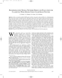
Standard Backpropagation (BP) The Backpropagation BP learns a predefined set of output example pairs by using a two–phase propagate adapts cycle. As seen in Figure 1, after an input pattern has been applied as a stimulus to first layer of network units, it is propagated through each upper layer until an output is generated. This output pattern is then compared to the desired output, and an error signal is computed for each output unit. The signals are then transmitted backward from the output layer to each unit in the intermediate layer that contributes directly to the output. However, each unit in the intermediate layer receives only a portion of the total error signal, based roughly on the relative contribution the unit made to the original output. This process repeats, layer by layer, until each unit in the network has received an error signal that describes its relative contribution to the total error.
Figure 1 - The Three-layer BP Architecture
We follow Freeman and Skapura’s book (1992) to describe the procedure of training feedforward neural networks using the backpropagation algorithm. The detailed formulas are described in the Appendix.
Optical Backpropagation (OBP) In this section, the adjustment of the new algorithm OBP (Otair & Salameh, 2004) will be described at which it would improve the performance of the BP algorithm. The convergence speed of the learning process can be improved significantly by OBP through adjusting the error, which will be transmitted backward from the output layer to each unit in the intermediate layer. In BP, the error at a single output unit is defined as: δo pk = (Ypk – O pk)
(1)
Where the subscript “P “refers to the pth training vector, and “K “refers to the kth output unit. In this case, Ypk is the desired output value, and Opk is the actual output from kth unit, then δpk will propagate backward to update the output-layer weights and the hidden-layer weights. While the error at a single output unit in adjusted OBP will be as:
168
Otair & Salameh
o
Newδ pk = (1 + e
(Y −O )2 pk pk
(2)
)
, if ( Ypk – O pk ) >= zero . o
Newδ pk = −(1 + e
(Y −O )2 pk pk
)
(3)
, if ( Ypk – O pk ) < zero. Where Newδ˚pk is considered as the new proposed in the OBP algorithm. An OBP uses two forms of Newδ˚pk, because the exp function always returns zero or positive values (and the adapts operation for many output units need to decrease the actual outputs rather than increasing it). This Newδ˚pk will minimize the errors of each output unit more quickly than the old δ˚pk, and the weights on certain units change very large from their starting values.
The steps of an OBP: 1. Apply the input example to the input units. 2. Calculate the net-input values to the hidden layer units. 3. Calculate the outputs from the hidden layer. 4. Calculate the net-input values to the output layer units. 5. Calculate the outputs from the output units. 6. Calculate the error term for the output units, but replace Newδ˚pk with δ˚pk (in all equations in appendix). 7. Calculate the error term for the output units, using Newδ˚pk, also. 8. Update weights on the output layer. 9. Update weights on the hidden layer. 10. Repeat steps from step 1 to step 9 until the error (Ypk – Opk) is acceptably small for each training vector pairs.
Proof: The output of BP and OBP for any output unit must be equal, if the BP output units multiply it by Factor (A), where (A) is defined as follows: A•
1 1+ e
−x
A = (1 + e
= (1 + e
(Y −O )2 pk pk
(Y −O )2 pk pk
) •1 + e
−x
)
(4)
(5)
The sigmoid function for each output unit in BP must be equal to the Newδ˚pk in OBP through multiplying it by this Factor. There is another way to find the factor (A) using the following assumptions:
169
Speeding Up Back-Propagation Neural Networks
Assumption 1: A1 •
1 1+ e
−x =
(1 + e
1 Y −O pk pk
(6) )
In other words, OBP uses a sigmoid function on each error of each output unit (Ypk – O pk), and it assumes that if the sigmoid function (on the left side in equation 6) is multiplied by (A1), it must be equal to those sigmoid function which applied on the error for the output units, then: A1 =
−x 1+ e Y −O pk pk (1 + e )
(7)
Assumption 2: An OBP assumes that if the sigmoid function – which is applied on the error of output units - is multiplied by (A2), then it must be equal to Newδ˚pk: A2•
1 Y −O pk pk ) (1+ e
(Y −O )2 pk pk ) = (1+ e
(8) A 2 = (1 + e
( Y −O ) pk pk
) • (1 + e
( Y −O ) 2 pk pk
)
(9)
Assumption 3: From equations (7) and (9), OBP assumed that: A = A1 * A2 = 1+ e
A = (1 + e
−x
(10) −x (Y −O ) (Y −O )2 1+ e pk pk pk pk • (1+ e ) • (1 + e ) (Y −O ) pk pk
) • (1 + e
Y −O pk pk 2 )
(11)
(12)
Comparative Study The OBP will be tested using the following real example that consider neural network with 6 units for input layer, 4 units for hidden layer, and 3 units for output layer. This example will train the network using OBP, and then it trains it using standard BP, and it compares the final results from OBP and BP. After the MSE (Mean Square Error) reached to 0.001 the training process discontinued. The initial weights selected randomly from –0.5 to +0.5, and the same initial weights have been used for the two algorithms. Learning rate equals to 0.01 has been taken in the training process Figure 2, shows the differences between the final weights from input layer to the hidden layer using an OBP, and BP are very small.
170
Otair & Salameh
Also, there are no huge differences between the two algorithms to adapt the weights from the hidden to the output layer. Figure (3) shows that:
The surprising results in the previous figure are the number of epochs using the two algorithms, which proves that the OBP is an optical algorithm if it is compared with the standard BP. This network was tested using the two algorithms using different learning rate, Table 1, shows the results.
Table 1– Training processes using different (η)
From Table1, it is observed that the results of OBP are much better and faster than the BP for all training processes with different learning rate.
Learning Rate (η)
Epochs
Epoch
Conclusion
0.01
1812
46798
This paper introduced a new algorithm OBP, which has been proposed for the training of multilayer neural networks, and it enhanced the version of the Backpropagation BP algorithm. The study shows that OBP is beneficial in speeding up the learning process. The simulation results confirmed these observations.
0.05
363
9351
0.1
182
4673
0.15
122
3114
0.2
92
2334
0.25
47
1866
OBP
BP
Training process defined as adapting weights for each 0.3 61 1554 unit in neural network, so the OBP is a good algorithm, because it can adapt all weights with optical time. The simulation results show that when a very small value is used for learning rate (η) with OBP makes the adapted final weights very closed become to the final weights that introduced from BP. So, it can escape from local minim.
Future Work Future work will test the proposed algorithm across a wide range of important problems and applications.
171
Speeding Up Back-Propagation Neural Networks
Appendix: Training a Feed Forward Neural Networks Using the Backpropagation Algorithm Assume there are m input units, n hidden units, and p output units. 1. Apply the input vector, Xp=(Xp1 , Xp2 , Xp3 ,….. , XpN )t to the input units . 2. Calculate the net- input values to the hidden layer units: N h net pj =( ∑ W h ji • X ) pi i =1
3. Calculate the outputs from the hidden layer: i pj = f
h
h j ( net pj )
4. Move to the output layer. Calculate the net-input values to each unit: net
O
L pk =( ∑ W O kj •i pj ) j =1
5. Calculate the outputs: O pk = f
o
o j ( net pk )
6. Calculate the error terms for the output units: o
δ pk = (Y pk − O pk ) • f
o′
o k ( net pk )
Where,
f o′ k (net o pk ) = f o k (net o pk ) • (1 − f o k (net o pk )) 7. Calculate the error terms for the hidden units M
δ h pj = f h′ j (net h pj ) • (∑ δ o pk • W o kj ) K =1
Notice that the error terms on the hidden units are calculated before the connection weights to the output-layer units have been updated. 8. Update weights on the output layer o o o W kj (t +1) = W kj (t ) + (η • δ pk • i pj )
9. Update weights on the Hidden layer W
h
ji (t +1) = W
h
h ji (t ) + (η • δ pj • X i)
References Callan, R. (1999). The Essence of Neural Networks, 33-52. Southampton Institute. Carling, A., (1992). Back propagation. Introducing Neural Networks, 133-154. Caudill, M. & Butler, C. (1993).Understanding neural networks. Computer Explorations, 1,155-218.
172
Otair & Salameh
Fahlman, S. E. (1988). Faster-learning variations on backpropagation: An empirical study. Proceedings of the 1988 Connectionist Models Summer School, 38-51. Freeman, J. A. &, Skapura, D. M. (1992). Backpropagation. Neural Networks Algorithm Applications and Programming Techniques, 89-125. Hagan, M. T. & Demuth, H. (1996). Neural Networks Design, 11.1-12.52. Hakin, S. (1999). Neural networks: A comprehensive foundation (2nd ed.). pp.161-184 Jacobs, R. A. (1988). Increased rates of convergence through learning rate adaptation. Neural Networks, 1, 169-180 Lee, Y., Oh, S. H., & Kim, M.W. (1991). The effect of initial weights on premature saturation in back propagation learning. Proceedings of the International Joint Conference on Neural Networks, Seattle, 1765-1770 Minai, A. A., & Williams, R. D (1990). Acceleration of back-propagation through learning rate momentum adaptation. Proceedings of the International Joint Conference on Neural Networks, 1676-1679. Otair, M. A. & Salameh, W. A. (2004). An improved back-propagation neural networks using a modified non-linear function. Proceedings of the IASTED International Conference, 2004, 442-447. Riedmiller, M & Braun, H. (1993). A direct adaptive method for faster backpropagation learning the PROP algorithm. Proceedings of the IEEE international conference on Neural Networks (ICNN), Vol. I, San Francisco, CA, 586-591. Rumelhart, D. E., Durbin, R. Golden, R., & Chauvin, Y. (1992). Backpropagation: Theoretical foundations. In Y.Chauvin & D. E Rumelhart (Eds.), Backpropagation and Connectionist Theory. Lawrence Erlbaum. Rumelhart, D. E., Hinton, G. E., & Williams, R. J. (1986). Learning internal representations by error propagation. In D. E. Rumelhart & J. L. McClelland (Eds.), Parallel Distributed Processing, pp. 318362.
Biographies Mohammed A. Otair is an Instructor of computer information systems, at the Jordan University of Science and Technology, IrbedJordan. He received his B.Sc. in Computer Science from IU-Jordan, and his M.Sc. and Ph.D in 2000, 2004, respectively, from the Department of Computer Information Sysems-Arab Academy. His major interests are Machine Learning, Neural Network Learning Paradigms, Web-computing, E-Learning.
Walid A. Salameh is an Associate Professor of computer Science, at the PSUT-RSS, Amman-Jordan. Hereceived his B.Sc. in Computer Science from YU-Jordan, and his M.Sc. and Ph.D in 1987, 1991, respectively, from the Department of Computer Engineering-METU. His major interests are Machine Learning, Neural Network Learning Paradigms, and Intelligent Learning Paradigm through the Web (Intelligent Web-learning based Paradigms).
173