Dynamic Energy Efficient Data Placement and Cluster Reconfiguration Algorithm for MapReduce Framework Nitesh Maheshwari∗, Radheshyam Nanduri, Vasudeva Varma Search and Information Extraction Lab Language Technologies Research Centre (LTRC) International Institute of Information Technology, Hyderabad (IIIT Hyderabad) Gachibowli, Hyderabad, India 500032
Abstract With the recent emergence of cloud computing based services on the Internet, MapReduce and distributed file systems like HDFS have emerged as the paradigm of choice for developing large scale data intensive applications. Given the scale at which these applications are deployed, minimizing power consumption of these clusters can significantly cut down operational costs and reduce their carbon footprint - thereby increasing the utility from a provider’s point of view. This paper addresses energy conservation for clusters of nodes that run MapReduce jobs. The algorithm dynamically reconfigures the cluster based on the current workload and turns cluster nodes on or off when the average cluster utilization rises above or falls below administrator specified thresholds, respectively. We evaluate our algorithm using the GridSim toolkit and our results show that the proposed algorithm achieves an energy reduction of 33% under average workloads and up to 54% under low workloads. Keywords: Energy Efficiency, MapReduce, Cloud Computing
∗
Corresponding author. Address: Search and Information Extraction Lab, Block B2, ”Vindhya”, International Institute of Information Technology, Gachibowli, Hyderabad 500 032, India. Tel.: +91-40-66531157. Email addresses:
[email protected] (Nitesh Maheshwari),
[email protected] (Radheshyam Nanduri),
[email protected] (Vasudeva Varma)
Preprint submitted to FGCS (Future Generation Computer Systems)
July 2011
1. Introduction Most enterprises today are focusing their attention on energy efficient computing, motivated by high operational costs for their large scale clusters and warehouses. This power related cost includes investment, operating expenses, cooling costs and environmental impacts. The U.S. Environmental Protection Agency (EPA) datacenter report [1] mentions that the energy consumed by datacenters has doubled in the period of 2000 and 2006 and estimates another two fold increase from 2007 to 2011 if the servers are not used in an improved operational scenario. A substantial percentage of these datacenters run large scale data intensive applications and MapReduce [2] has emerged as an important paradigm for building such applications. MapReduce framework, by design, incorporates mechanisms to ensure reliability, load balancing, fault tolerance, etc. but such mechanisms can have an impact on energy efficiency as even idle machines remain powered on to ensure data availability. The Server and Energy Efficiency Report [3] states that more than 15% of the servers are run without being used actively on a daily basis. Consider the case of a website for which the traffic is not uniform throughout the year. The website owners can either invest in buying more servers or move to a cloud platform. Moving to cloud is clearly a better alternative for the website owners as they can add resources based on the traffic according to a pay-per-use model. But for cloud computing to be efficient, the individual servers that make up the datacenter cloud will need to be used optimally. None of the major cloud providers release their server utilization data, so it is not possible to know how efficient cloud computing actually is. We have also observed that most applications developed today fail to exploit the low power modes supported by the underlying framework. In this paper, we address the issue of power conservation for clusters of nodes that run MapReduce jobs, as there is no separate power controller in MapReduce frameworks such as Hadoop [4]. Although we focus on one specific framework, our approach can also be applied to other application frameworks where the framework’s power controller module can be connected to its foundational software. Our key contribution is an algorithm that dynamically reconfigures the cluster based on the current workload. It scales up (down) the number of nodes in the cluster when the average cluster utilization rises above (falls below) a threshold specified by the cluster administrator. By doing this the nodes in the cluster that are underutilized can be turned off 2
to save power. We remodel the cluster’s data placement policy to place the data on the cluster and reconfigure the cluster depending on the workload experienced. The advantage of such a modification to the framework is that the applications developed for these clusters need not be fine-tuned to be energy aware. To verify the efficacy of our algorithm, we simulated the Hadoop Distributed File System (HDFS) [5] using the GridSim toolkit [6]. We studied the behavior of our algorithm with the default Hadoop implementation as baseline and our results indicate an energy reduction of 33% under average workloads and up to 54% under low workloads. A substantial amount of earlier research has dealt with optimizing the energy efficiency of servers at a component level like processors, memories and disks [7, 8, 9, 10]. Most literature in this field focuses on solving the problem of energy efficiency using local techniques like Dynamic Voltage Scaling (DVS), request batching and multi-speed disks [11, 12, 13]. In our work, we employ the use of a cluster wide technique where the global state of the cluster is used to dynamically scale the cluster to handle the workload imposed on it. The remainder of this paper is organized as follows. We give a brief overview of HDFS rack aware data placement policy and the key idea behind our chosen approach in Section 2. Next, we present our energy efficient algorithm for cluster reconfiguration and data placement in Section 3. Section 4 describes the methodology and simulation models used in evaluating our algorithm and the results of evaluation. We then compare our work with existing work in Section 5. Finally, we conclude by summarizing the key contributions, and touching on future topics in this area in Section 6. 2. Background 2.1. Need for a Power Controller in MapReduce With the emergence of cloud computing in the past few years, MapReduce [2] has seen tremendous growth especially for large-scale data intensive computing [14]. A large segment of this MapReduce workload is managed by Hadoop [4], Amazon Elastic MapReduce [15] and Google’s in house MapReduce implementation. MapReduce was designed for deployment on clusters running inexpensive commodity hardware. Hence, even idle nodes remain powered on to ensure data availability. However, there is no separate power controller in MapReduce frameworks such as Hadoop as yet. 3
100
Server power usage (percent of peak)
90 80 70 60 50 40 30
Power
20
Energy Efficiency
10 0 0
10
20
30
40
50
60
70
80
90
100
Utilization (percent)
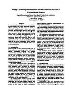
Figure 1: Server power usage and energy efficiency at varying utilization levels, from idle to peak performance. Even an energy-efficient server still consumes about half its full power when doing virtually no work. Source: [16]. Datacenters are known to be expensive to operate and they consume huge amounts of electric power [17]. Google’s server utilization and energy consumption study [16] reports that the energy efficiency peaks at full utilization and significantly drops as the utilization level decreases (Figure 1). Hence, the power consumption at zero utilization is still considerably high (around 50%). Essentially, even an idle server consumes about half its maximum power. We also observe that the energy efficiency of these servers lies in the range of 20-60% when operating under 20-50% utilization. Thus Figure 1 indicates that dynamically reconfiguring the cluster by scaling it while running the active nodes at higher utilization is the best decision from a power management point of view. The MapReduce framework implemented by Hadoop relies heavily on the performance and reliability of the underlying HDFS. It divides applications into numerous smaller blocks of work and application data into smaller data blocks. It then allows parallel execution for applications in a fault tolerant way by creating redundant copies of both data and computation.
4
2.2. HDFS Data Layout HDFS is based on Google File System (GFS) [18] and has a master-slave architecture with the master called as NameNode and the slaves as DataNodes. The NameNode is responsible for storing the HDFS namespace and records changes to the file system metadata. The DataNodes are spread across multiple racks and store the HDFS data in their local file systems as shown in Figure 2. The DataNodes are connected via a network and intrarack network bandwidth between machines is usually higher than interrack network bandwidth. Worker Nodes (DataNodes)
Racks
Heartbeats Data blocks
Master (NameNode) Data Files
Figure 2: Architecture of Hadoop Distributed File System (HDFS). The communication between the master node (NameNode) and the worker nodes (DataNodes) is shown by means of Heartbeat messages. The files to be stored on HDFS are split in 64 MB chunks and distributed across racks. Each file stored on HDFS is split into smaller chunks of size 64 MB called data blocks and these blocks are distributed across the cluster. Each block is replicated to ensure data availability even in case of connectivity failure 5
to nodes or even complete racks. For the same, Hadoop implements a rackaware data block replication policy for the data that is stored on HDFS. For the default replication factor of three, HDFS’s replica placement policy is to put one replica of the block on one node in the local rack, another on a different node in the same rack, and the third on a node in some other rack. Each DataNode periodically sends a heartbeat message to the NameNode in order to inform the NameNode about its current state including the block report of the blocks it stores. The NameNode assumes DataNodes without recent heartbeat messages to be dead and stops forwarding any more requests to them. The NameNode also re-replicates the data lost because of dead nodes, corrupt blocks, hard disk failures, etc. If some DataNodes are turned off without informing the NameNode then the cluster might enter what can be called as a panic phase where the NameNode tries to replicate the blocks earlier stored on these DataNodes. This process might end up generating heavy network traffic [19]. 2.3. Replica Placement in Hadoop Racks
DataNodes
Data block to be placed First Replica Second Replica Third Replica
Figure 3: A typical replica pipeline in Hadoop for a replication factor of 3. In the context of high-volume data processing, the limiting factor is the rate at which data can be transferred between nodes. Hadoop uses the bandwidth between the nodes as a measure of distance between them. Hence, the cost of data transfer between nodes in the same rack is less than that of 6
nodes in different racks, which in turn is less than that of nodes on different datacenters. Replication pipeline for a replication factor of three is shown in Figure 3. 3. Proposed Algorithm We attempt to reduce the energy consumption of datacenters that run MapReduce jobs by reconfiguring the cluster. In this section, we explain the approach followed in our proposed algorithm for cluster reconfiguration. 3.1. Approach We implement a channel between the cluster’s power controller and HDFS that scales the number of nodes in the cluster dynamically to meet the current service demands (Figure 4). We start with a subset of nodes powered on and intelligently accept job requests by checking if they can be served using the current state of the cluster. We add more nodes to the cluster if the resources available are not enough for serving these requests. We power them off again when they are not being used optimally. When the NameNode receives a request to create a file Fk of size Sk with replication factor of Rk , it calculates the number of HDFS blocks that will be needed to store it using the following formula: dSk /Be × Rk
(1)
where B is the HDFS block size. The block size is configurable per file with a default value of 64 MB. The space needed to store Fk on HDFS is: Sk × Rk
(2)
The algorithm checks if the there is enough space available on HDFS to store the file and turns on more nodes if needed. At all times, we keep some space reserved on the DataNodes so that write operations do not block or fail waiting for more space to be provisioned while new DataNodes are being powered on. After the nodes are powered on, the cluster is rebalanced as there is no data on the newly activated DataNodes while other DataNodes are already filled substantially. The NameNode gives instructions to the DataNodes to create blocks in a rack-aware manner on HDFS and updates its namespace and metadata.
7
When the NameNode receives a request to delete a file, it gives instructions to the DataNodes to delete blocks corresponding to that file. This communication with the DataNodes happens by means of heartbeat messages that are exchanged periodically between the NameNode and the DataNodes. If the cluster becomes underutilized after deleting the data, we move the data from the least utilized nodes to other nodes and turn them off. We shall make use of the following notation in the rest of the paper: • n = Number of currently active nodes on the cluster • Cθ = Disk capacity of DataNode θ • Uθ = Current utilization of DataNode θ • Rθ = Set of active nodes in DataNode θ’s rack • U = Average utilization of active nodes in the cluster • U (R) = Average utilization of active nodes in rack R • Uu = Scale up threshold • Ud = Scale down threshold • τ = Transfer threshold (in percentage) • δ = Dampening factor for interrack transfer (in percentage) • λ = Percentage of initially inactive nodes per rack • µ = Minimum percentage of active nodes per rack All the U values mentioned above are in percentage. As demonstrated in Figure 4, when the NameNode receives a request to create a file, it checks with the Power Controller if there is a need to scale up the cluster to accommodate the current request. Similarly, when some data is deleted from the cluster, the NameNode consults the Power Controller if some nodes can be deactivated to save power. The Power Controller module responds with cluster reconfiguration information which has details about the nodes to be activated or deactivated. It decides which nodes to activate or deactivate based on scale up threshold Uu , scale down threshold Ud and the current average utilization of active nodes in the cluster U . 8
Racks U(R1)
DataNodes U(R2)
U(Rk)
Rebalancing & Scaling
NameNode Need to scale up/down? Ud
U
Reconfiguration information
Power Controller
Uu
Figure 4: Proposed Approach: Interaction of Power Controller module with the NameNode. The NameNode performs Rebalancing and Scaling operations once it receives the reconfiguration information from the Power Controller. Once this cluster reconfiguration information is received by the NameNode, it performs scaling and rebalancing operations depending on the average utilization U (Ri ) of active nodes in racks. A detailed description of these operations is covered in subsequent sections. The latest version of Hadoop (0.21.0) comes with a pluggable interface to place replicas of data blocks in HDFS and has support for an API that allows a module external to HDFS to specify how data blocks should be placed [20]. This will ease the integration of placement policy we suggest in Hadoop. 3.2. Cluster Reconfiguration We consider the following types of cluster reconfigurations in our approach.
9
3.2.1. Scaling Up Figure 5 presents our algorithm for scaling up the cluster when the current state of resources are not enough to serve write requests. Scaling up of the cluster is triggered when the average utilization of the active nodes (U ) exceeds the administrator specified threshold Uu . 1: 2: 3: 4: 5: 6: 7: 8: 9: 10: 11: 12: 13: 14: 15: 16: 17: 18: 19: 20: 21:
if U > Uu then ActivateDataN odes(Θ) for all θdst ∈ Θ do for all θsrc ∈ [Rθdst − θdst ] do {For all nodes in the same rack} if Uθsrc − U > τ then p = (Uθsrc − U ) × Cθsrc IntrarackT ransf er(θsrc , θdst , p) end if end for if Uθdst < U (Rθdst ) then for all θsrc ∈ / Rθdst do {For all nodes in some other rack} if Uθsrc − U > τ then p = (Uθsrc − U − δ) × Cθsrc InterrackT ransf er(θsrc , θdst , p) end if end for end if end for end if
Figure 5: Algorithm for Scaling Up reconfiguration. Upon reaching the trigger condition, we perform intrarack transfer and interrack transfer to all the newly added nodes. When the trigger condition is reached, we select a set of DataNodes (Θ) to be powered on in the function ActivateDataN odes(Θ). We choose the least recently deactivated nodes to avoid hotspots caused by the same set of machines running all the time. It is advantageous to activate nodes from different racks because HDFS follows a rack-aware replica placement policy where replicas of a data block are spread across multiple racks. Also, acti10
vating multiple nodes in the same iteration saves time as these nodes can be booted in parallel. Addition of new nodes while scaling up will result in more storage space on the cluster. As a result of this, the average utilization level of the cluster will drop and the data distribution across nodes will become skewed. Therefore, we balance the racks where new nodes were recently activated. For each newly activated DataNode (θdst ) we first perform intrarack transfer of blocks (Figure 5, lines 4 to 10). If the utilization of a node (θsrc ) in the rack exceeds U by the transfer threshold (τ ) specified by the administrator, we transfer the excess amount of data from θsrc to θdst . If the intrarack transfer does not sufficiently fill up the storage on θdst , interrack transfer of blocks to θdst is performed (Figure 5, lines 12 to 18). Since interrack transfer is costlier than intrarack transfer, the amount of excess data to be moved in case of interrack transfer is hindered by a value of δ. 3.2.2. Scaling Down Figure 6 presents our algorithm for scaling down the cluster. Scaling down of the cluster is triggered when the average utilization of the active nodes (U ) falls below the administrator specified threshold Ud . If the trigger condition is reached, it is likely that some nodes in the cluster are underutilized. Time of activation and current utilization of nodes are considered in function CandidateSet() while selecting the set of candidate nodes (Θ) that can potentially be powered off. We perform two checks on each candidate node (θsrc ) before deactivating it. Firstly, we do not deactivate a node if some node from its rack has been deactivated recently. Secondly, we keep a percentage of nodes (µ) activated at all times in all the racks so that the cluster can still serve write requests that are received in bursts. For each candidate node θsrc , we calculate the expected average utilization of its rack (m0 ) if θsrc was to be powered off. We then perform intrarack transfer of blocks to nodes in the same rack (Figure 6, lines 6 to 12). If the difference between Uθdst and m0 is less than the transfer threshold specified (τ ) by the administrator, we transfer the excess amount of data from θsrc to θdst . If the intrarack transfer does not completely vacate the storage on θsrc , interrack transfer of blocks from θsrc is performed (Figure 6, lines 14 to 20). As in the case of scaling up reconfiguration, the amount of excess data to be moved in case of interrack transfer is hindered by a value of δ. When all the data blocks from θsrc have been moved, we add it to the set of nodes 11
1: 2: 3: 4: 5: 6: 7: 8: 9: 10: 11: 12: 13: 14: 15: 16: 17: 18: 19: 20: 21: 22: 23: 24: 25:
if U < Ud then Σ ← ∅ {Set of nodes that will be deactivated} Θ = CandidateSet() for all θsrc ∈ Θ do m0 = (U (Rθsrc ) × |Rθsrc |)/(|Rθsrc | − 1) for all θdst ∈ [Rθsrc − θsrc ] do {For all nodes in the same rack} if Uθdst − m0 < τ then p = (m0 + δ − Uθdst ) × Cθdst IntrarackT ransf er(θsrc , θdst , p) end if end for if Uθsrc > 0 then for all θdst ∈ / Rθsrc do {For all nodes in some other rack} if Uθdst − m0 < τ then p = (m0 − Uθdst ) × Cθdst InterrackT ransf er(θsrc , θdst , p) end if end for end if Σ ← Σ ∪ θsrc end for DeactivateDataN odes(Σ) end if
Figure 6: Algorithm for Scaling Down reconfiguration. Upon reaching the trigger condition, we perform intrarack transfer and interrack transfer from the nodes to be removed.
12
to be deactivated (Σ). Finally, after considering all the candidate nodes, we deactivate the nodes in Σ. 3.2.3. Avoiding Jitter Effect While performing these scaling operations of activating and deactivating the nodes in the cluster, the cluster can experience a jitter effect if the load variability is high. Consider a case when by the time new nodes were being activated, the load dissipates resulting in shutting down some already activate nodes, at which time the load was increasing again. The parameters for our algorithm can be configured in a way that this jitter effect does not occur. The difference in the values of scale up threshold Uu and scale down threshold Ud should be made sufficiently large so that the cluster does not experience a jitter effect of activating and deactivating nodes due to small changes in average utilization of active nodes in the cluster U . 3.3. Cluster Rebalancing The level of network activity depends on the techniques used for rebalancing the cluster; hence they are very crucial for our algorithm to perform well. The cluster needs to be rebalanced after scaling up the number of nodes in the cluster in order to distribute the extra workload from overutilized nodes to the newly added nodes. Similarly, we need to perform rebalancing operations before scaling down the number of nodes in the cluster so that workload from underutilized nodes can be transferred to already active nodes before they can be turned off. We put an upper limit on the bandwidth used for rebalancing operations so that it does not congest the network. This also ensures that the other ongoing file operations remain unaffected while the cluster is being rebalanced. We employ a simple heuristic for rebalancing where we try to move the maximum amount of data to nodes in the same rack as network bandwidth is greater for intrarack transfers. While moving data blocks across nodes, we do not violate the rack-aware replica placement policy followed by HDFS. We also do not move data that is currently being used by some job already running on the cluster. This ensures that we do not compromise on the fault tolerance and runtime of already running jobs on the cluster while performing rebalancing operations. A data block is removed from the source DataNode only after all the running tasks using that data block are completed. In order to respect the rack aware block replication policy followed by Hadoop, we
13
make the following checks before moving a data block within the same rack and across racks (Figure 7 explains this approach by means of examples): Data Blocks Interrack transfers
Intrarack transfers
DataNode
Rack Valid Transfers
Invalid Transfers
Figure 7: Examples of valid and invalid movement of data blocks while performing intrarack and interrack transfer.
Intrarack Transfer : Intrarack transfer means transferring a data block from a node to some other node in the same rack. While performing intrarack transfer, we move a data block from a node to another node only if a replica of that block does not exist on the destination node. Nodes in the same rack are connected by a higher bandwidth link and hence intrarack transfers are cheaper as compared to interrack transfers. Interrack Transfer : Interrack transfer means transferring a data block from a node to one of the nodes in some other rack. In the case of interrack transfer, a data block is moved from a node to another node only if a replica of that block does not exist on any nodes in the destination rack. 14
The subroutines IntrarackT ransf er(θsrc , θdst , p) and InterrackT ransf er(θsrc , θdst , p) in the algorithms of Figure 5 and 6 transfer p amount of data from node θsrc to node θdst . Table 1 summarizes the amount of data transferred from θsrc to θdst for intrarack and interrack transfers while scaling up and scaling down operations. Scaling Up
Scaling Down
1
Intrarack (Uθsrc − U ) × Cθsrc Transfer
(m0 + δ − Uθdst ) × Cθdst
Interrack (Uθsrc −U −δ)×Cθsrc Transfer
(m0 − Uθdst ) × Cθdst
Table 1: Data transferred (p) from θsrc to θdst
4. Evaluation and Results We use the GridSim toolkit to simulate HDFS architecture and perform our experiments. We verify the efficacy of our algorithm and study its behavior with the default HDFS implementation as baseline. 4.1. Simulation Model The NameNode and DataNode classes in our simulations are extended from the GridSim toolkit’s DataGridResource class. These DataNodes are distributed across racks and a metadata of these mappings is maintained at the NameNode. We implement the default rack-aware replica placement policy followed by HDFS. We then incorporate the cluster reconfiguration decisions suggested by our algorithm to dynamically scale the number of nodes in the cluster. We demonstrate the scale up and scale down operations of our algorithm and their corresponding energy savings. The parameters used in our simulation runs along with their default values are specified in Table 2. These parameters are kept constant at their default values between different runs while comparing the results. All values reported in these results are averaged over ten independent runs of varying workloads, 1
where m0 =
U (Rθsrc )×|Rθsrc | |Rθsrc |−1
15
Table 2: Simulation Parameters Parameter
Description
Number of racks
U nif ormRandom(5, 10) [Def ault = 8]
Number of nodes per rack
U nif ormRandom(10, 20) [Def ault = 15]
Storage capacity of nodes (GB)
U nif ormRandom(100, 500)
HDFS default block size, B
64 MB
Scale up threshold, Uu
80%
Scale down threshold, Ud
50%
Transfer threshold, τ
5%
Dampening factor for interrack transfer, δ
5%
Percentage of initially inactive 30-70% [Def ault = 50] nodes per rack, λ Minimum percentage of active nodes per rack, µ
30-70% [Def ault = 50]
unless otherwise specified. We vary the number, size and replication factor of the files created on the HDFS in our experiments. 4.2. Cluster Reconfiguration To verify whether our cluster reconfiguration algorithm is able to scale the cluster in accordance to the workload imposed on it, we perform basic experiments for scale up and scale down operations. These experiments were performed with 50 nodes spread across 5 racks, with each rack having 10 nodes. We plot the number of active nodes and their average utilization for the default HDFS implementation and our algorithm, when presented with the same workload (Figure 8a and 8b). 4.2.1. Scaling Up Figure 8a summarizes the results of our scale up experiments. We start with a percentage of nodes (λ = 50%) turned off initially and scale up the 16
90
90
80
80
70
70
60
60
50
50
40
40
30
30
20
20
10
10 0
0 0
25
50
75
100
125
150
175
200
Percentage Utilization of active nodes
Number of active nodes
Percentage Utilization (Default HDFS) Number of active nodes (Default HDFS) Number of active nodes (Our algorithm) Percentage Utilization (Our algorithm)
Simulation time
Number of active nodes
Percentage Utilization (Default HDFS) Number of active nodes (Default HDFS) Number of active nodes (Our algorithm) Percentage Utilization (Our algorithm) 90
90
80
80
70
70
60
60
50
50
40
40
30
30
20
20
10
10
0
0 0
25
50
75
100
125
150
175
200
Percentage Utilization of active nodes
(a) Basic scale up operation, with Uu = 80% and λ = 50%
Simulation time
(b) Basic scale down operation, with Ud = 50% and µ = 50%
Figure 8: Basic Scale Up and Scale Down operations for a cluster of 50 nodes spread across 5 racks, with each rack having 10 nodes.
17
cluster when the average utilization rises above the scale up threshold (Uu = 80%). The boxed area in the plot represents the scaling up operation where more nodes are added to the cluster whenever the cluster utilization (U ) rises above the value Uu . Adding more nodes to the cluster brings down the average utilization of the nodes in the cluster and it accepts incoming requests until the average utilization reaches Uu again, as demonstrated by the peaks in the curve (Figure 8a). Our algorithm tries to maintain the utilization levels of the nodes at Uu affirming that the nodes are being used in the region of higher energy efficiency, as specified in Figure 1. In this case, the average number of inactive nodes during the experiments denote energy savings of about 36%. 4.2.2. Scaling Down Figure 8b summarizes the results of our scale down experiments. Initially all the nodes in the cluster are being used and we scale down the cluster when the average utilization falls below the scale down threshold (Ud = 50%). The boxed area in the plot represents the scaling down operation where nodes are deactivated from the cluster whenever the cluster utilization (U ) falls below the value Ud . Deactivating nodes from the cluster brings up the average utilization of the nodes and our algorithm scales down the cluster till the percentage of active nodes is more than the value specified by µ, as demonstrated by the curve in Figure 8b. The energy savings denoted by the experiments in this case is about 27%. 4.3. Energy Savings Next, we perform scale up and scale down experiments over a range of workloads to calculate the average energy savings with our algorithm. These experiments were performed with 120 nodes spread across 8 racks, with each rack having 15 nodes. In our model, the amount of energy saved is proportional to the number of deactive nodes. We plot the energy savings for the cases when the cluster is imposed with low and high workloads. 4.3.1. Workload Imposed The number of files is varied from 200 for low workloads to 400 for high workloads and the minimum file size is varied from 3000 MB for low workloads to 15000 MB for high workloads. The maximum file size is set to 25000 MB across all the experiments, whereas the number of replicas of these files is selected randomly from 1 to 3. We observe that the cluster intelligently 18
reconfigures itself based on the workload imposed, proving the effectiveness of our algorithm. As expected, the energy conserved in case of low workloads is significantly higher. 4.3.2. Scaling Up and the effect of λ We calculate the average amount of energy saved during the scale up operation by performing experiments over a range of various workloads (Figure 9). We analyze the behavior of the plots for various values of λ, which is the percentage of nodes kept inactive at the start of each experiment. The average energy savings denoted by these experiments is about 36%.
Energy savings (in percentage)
60
54.66
52.49 50
44.05 38.24
40 30
26.35
35.76 26.98
20
37.89
30.48
19.87 Low workload
10
High workload 0 30
40
50
60
Percentage of initially inactive nodes, λ
70
Figure 9: The effect of varying λ on energy savings while scaling up We make the following observations from the plots: • Increasing the value of λ increases the percentage of energy conserved. • Energy conserved for low workloads can reach up to 54% for higher values of λ. • Even for high workloads and lower values of λ, the energy conserved is about 20%.
19
4.3.3. Scaling Down and the effect of µ We calculate the average amount of energy saved during the scale down operation in a similar manner over a range of various workloads (Figure 10). We analyze the behaviour of the plots for various values of µ, which is the minimum percentage of nodes that must be kept active in each rack at all times. The average energy savings denoted by these experiments is about 30%.
Energy savings (in percentage)
60 Low workload 50
48.43 43.58
High workload
41.95
40
35.15
32.80
30 20
26.76
23.70
22.11
18.22
10
15.68
0 30
40
50
60
70
Minimum percentage of active nodes per rack, μ
Figure 10: The effect of varying µ on energy savings while scaling down We then make the following observations from the plots: • Increasing the value of µ decreases the percentage of energy conserved. • Energy conserved for low workloads can reach up to 48% for lower values of µ. • Even for high workloads and higher values of µ, the energy conserved is about 15%. 5. Related Work Lowering the energy usage of datacenters is a challenging and complex issue because computing applications and data are growing so quickly that increasingly larger servers and disks are needed to process them fast enough 20
within the required time period [21]. Fan et al. report that the opportunities for power and energy savings are significant at the cluster-level and hence the systems need to be energy efficient across their activity range [22]. For MapReduce frameworks like Hadoop Vasi´c et al. present a design for energy aware MapReduce and HDFS where they leverage the sleeping state of machines to save power [19]. Their work also proposes a model for collaborative power management where a common control platform acts as a communication channel between the cluster power management and services running on the cluster. Leverich et al. present a modified design for Hadoop that allows scale-down of operational cluster [23]. They propose the notion of covering subset during block replication that at least one replica of a data block must be stored in the covering subset. This ensures data availability, even when all the nodes not in the covering subset are turned off. Also, the system configuration parameters used for MapReduce clusters have a high impact on their energy efficiency [24]. An important difference between the works mentioned above and our work is that the techniques employed in these works compromise on the replication factor of data blocks stored on the cluster. Our algorithm attempts to keep the cluster utilized to its maximum allowed potential and accordingly scale the number of nodes without compromising on the replication factor for the data blocks. Our work is inspired from earlier works by Pinheiro et al. where they present the problem of energy efficiency using cluster reconfiguration at the application level for clusters of nodes, and at the operating system level for standalone servers [25, 26]. We present the same problem for a cluster of machines running MapReduce frameworks such as Hadoop. Work by P´erez et al. in [27] presents a mathematical formalism to achieve dynamic reconfiguration with the use of storage groups for data-based clusters. Work by Duy et al. also presents this problem using machine learning based approach by applying the use of neural network predictors to predict future load demand based on historical demand [28]. The technique of Dynamic Voltage Scaling (DVS) has been employed to provide power-aware scheduling algorithms to minimize the power consumption [29, 30]. DVS is a power management technique where undervolting (decreasing the voltage) is done to conserve power and overvolting (increasing the voltage) is done to increase computing performance. Hsu et al. apply a variation of DVS called Dynamic Voltage Frequency Scaling (DVFS) by operating servers at various CPU voltage and frequency levels to reduce overall 21
power consumption [31]. Berl et al. propose virtualization with cloud computing as a way forward to identify the main sources of energy consumption [32]. Live migration and placement optimizations of virtual machines (VM) have been used in earlier works to provide a mechanism to achieve energy efficiency [33, 34, 35]. Power aware provisioning and scheduling of VMs has also been used with DVFS techniques to reduce the overall power consumption [36, 37]. Although virtualization helps reduce datacenter’s power consumption, the ease of provisioning virtualized servers can lead to uncontrolled growth and more unused servers, a phenomenon called virtual server sprawl [3]. 6. Conclusion and Future Work In this paper we addressed the problem of energy conservation for large datacenters that run MapReduce jobs. We also discussed that servers are most efficient when used at a higher utilization level. In this context, we proposed an energy efficient data placement and cluster reconfiguration algorithm that dynamically scales the cluster in accordance with the workload imposed on it. However, the efficacy of this approach would depend on how quickly a node can be activated. We evaluated our algorithm by performing simulations and the results show energy savings of as high as 54% under low workloads and about 33% under average workloads. Future directions of our research include applying machine learning approaches to study the resource usage patterns of jobs and model their power usage characteristics to efficiently schedule them on the cluster. Upon submission of a job, make use of the knowledge about the dataset to predict the data layout for its data blocks and optimally schedule the tasks making use of data locality. We would also like to study the performance of our algorithm when presented with different types of workloads such as processor intensive, memory intensive, disk intensive and network intensive. We would also like to study the impact of node’s boot time and ACPI [38] power states available in the hardware on the efficiency of our algorithm. We plan to find optimal values of MapReduce configuration parameters so that our algorithm can provide even better energy savings. We also plan to make use of multiple heuristics like access time and minimum replication factor of a file, while rebalancing the cluster to avoid overhead on the network.
22
Acknowledgment This work is partly supported by a grant from Yahoo! India R&D, under the Nurture an area: Cloud Computing project. We would like to thank Chidambaran Kollengode of Yahoo! and Reddyraja Annareddy of Pramati Technologies for their continual guidance throughout this work. We would also like to thank Jaideep Dhok, Sudip Datta and Manisha Verma for their constant feedback on our work. References [1] EPA report to Congress on Server and Data Center Energy Efficiency, Tech. rep., U.S. Environmental Protection Agency (2007). [2] J. Dean, S. Ghemawat, Mapreduce: simplified data processing on large clusters, Commun. ACM 51 (1) (2008) 107–113. doi:http://doi.acm.org/10.1145/1327452.1327492. [3] Server Energy and Efficiency Report, Tech. rep., 1E (2009). [4] Apache Hadoop, http://hadoop.apache.org. [5] Hadoop Distributed File System, http://hadoop.apache.org/hdfs/. [6] R. Buyya, M. Murshed, Gridsim: a toolkit for the modeling and simulation of distributed resource management and scheduling for grid computing, Concurrency and Computation: Practice and Experience 14 (2002) 1175–1220. doi:http://dx.doi.org/10.1002/cpe.710. [7] M. Weiser, B. Welch, A. Demers, S. Shenker, Scheduling for reduced cpu energy, in: OSDI ’94: Proceedings of the 1st USENIX conference on Operating Systems Design and Implementation, USENIX Association, Berkeley, CA, USA, 1994, p. 2. [8] A. Rangasamy, R. Nagpal, Y. Srikant, Compiler-directed frequency and voltage scaling for a multiple clock domain microarchitecture, in: CF ’08: Proceedings of the 5th conference on Computing frontiers, ACM, New York, NY, USA, 2008, pp. 209–218. doi:http://doi.acm.org/10.1145/1366230.1366267.
23
[9] A. R. Lebeck, X. Fan, H. Zeng, C. Ellis, Power aware page allocation, in: ASPLOS-IX: Proceedings of the ninth international conference on Architectural support for programming languages and operating systems, ACM, New York, NY, USA, 2000, pp. 105–116. doi:http://doi.acm.org/10.1145/378993.379007. [10] D. P. Helmbold, D. D. Long, T. L. Sconyers, B. Sherrod, Adaptive disk spindown for mobile computers, Mobile Networks and Applications 5 (2000) 285–297. [11] M. Elnozahy, M. Kistler, R. Rajamony, Energy conservation policies for web servers, in: USITS’03: Proceedings of the 4th conference on USENIX Symposium on Internet Technologies and Systems, USENIX Association, Berkeley, CA, USA, 2003. [12] E. V. Carrera, E. Pinheiro, R. Bianchini, Conserving disk energy in network servers, in: ICS ’03: Proceedings of the 17th annual international conference on Supercomputing, ACM, New York, NY, USA, 2003, pp. 86–97. doi:http://doi.acm.org/10.1145/782814.782829. [13] S. Gurumurthi, A. Sivasubramaniam, M. Kandemir, H. Franke, Drpm: Dynamic speed control for power management in server class disks, Computer Architecture, International Symposium on 0 (2003) 169. doi:http://doi.ieeecomputersociety.org/10.1109/ISCA.2003.1206998. [14] J. Dhok, N. Maheshwari, V. Varma, Learning based opportunistic admission control algorithm for mapreduce as a service, in: ISEC ’10: Proceedings of the 3rd India software engineering conference, ACM, 2010, pp. 153–160. doi:http://doi.acm.org/10.1145/1730874.1730903. [15] Amazon Elastic MapReduce, http://aws.amazon.com/elasticmapreduce/. [16] L. Barroso, U. Holzle, The case for energy-proportional computing, Computer 40 (12) (2007) 33 –37. doi:10.1109/MC.2007.443. [17] R. Buyya, C. S. Yeo, S. Venugopal, J. Broberg, I. Brandic, Cloud computing and emerging it platforms: Vision, hype, and reality for delivering computing as the 5th utility, Future Generation Computer Systems 25 (6) (2009) 599 – 616. doi:DOI: 10.1016/j.future.2008.12.001.
24
[18] S. Ghemawat, H. Gobioff, S.-T. Leung, The google file system, SIGOPS Oper. Syst. Rev. 37 (5) (2003) 29–43. doi:http://doi.acm.org/10.1145/1165389.945450. [19] N. Vasi´c, M. Barisits, V. Salzgeber, D. Kostic, Making cluster applications energy-aware, in: ACDC ’09: Proceedings of the 1st workshop on Automated control for datacenters and clouds, ACM, New York, NY, USA, 2009, pp. 37–42. doi:http://doi.acm.org/10.1145/1555271.1555281. [20] [HDFS-385] Design a pluggable interface to place replicas of blocks in HDFS, https://issues.apache.org/jira/browse/HDFS-385. [21] R. Buyya, A. Beloglazov, J. H. Abawajy, Energy-efficient management of data center resources for cloud computing: A vision, architectural elements, and open challenges, CoRR abs/1006.0308. [22] X. Fan, W.-D. Weber, L. A. Barroso, Power provisioning for a warehouse-sized computer, in: ISCA ’07: Proceedings of the 34th annual international symposium on Computer architecture, ACM, New York, NY, USA, 2007, pp. 13–23. doi:http://doi.acm.org/10.1145/1250662.1250665. [23] J. Leverich, C. Kozyrakis, On the energy (in)efficiency of hadoop clusters, SIGOPS Oper. Syst. Rev. 44 (1) (2010) 61–65. doi:http://doi.acm.org/10.1145/1740390.1740405. [24] Y. Chen, T. X. Wang, Energy efficiency of map reduce (2008). [25] E. Pinheiro, R. Bianchini, E. V. Carrera, T. Heath, Load balancing and unbalancing for power and performance in cluster-based systems (2001). [26] E. Pinheiro, R. Bianchini, E. V. Carrera and T. Heath, Dynamic cluster reconfiguration for power and performance, in: Power and energy management for server systems, IEEE Computer Society, 2004. [27] M. S. P´erez, A. S´anchez, J. M. Pena, V. Robles, A new formalism for dynamic reconfiguration of data servers in a cluster, Journal of Parallel and Distributed Computing 65 (10) (2005) 1134 – 1145, design and Performance of Networks for Super-, Cluster-, and Grid-Computing Part I. doi:DOI: 10.1016/j.jpdc.2005.04.018. 25
[28] T. V. T. Duy, Y. Sato, Y. Inoguchi, Performance evaluation of a green scheduling algorithm for energy savings in cloud computing, Parallel Distributed Processing, Workshops and Phd Forum (IPDPSW), 2010 IEEE International Symposium on (2010) 1 – 8doi:10.1109/IPDPSW.2010.5470908. [29] K. H. Kim, R. Buyya, J. Kim, Power Aware Scheduling of Bag-ofTasks Applications with Deadline Constraints on DVS-enabled Clusters, in: Cluster Computing and the Grid, 2007. CCGRID 2007. Seventh IEEE International Symposium on, 2007, pp. 541 –548. doi:10.1109/CCGRID.2007.85. [30] Y. C. Lee, A. Y. Zomaya, Minimizing energy consumption for precedence-constrained applications using dynamic voltage scaling, in: CCGRID ’09: Proceedings of the 2009 9th IEEE/ACM International Symposium on Cluster Computing and the Grid, IEEE Computer Society, Washington, DC, USA, 2009, pp. 92–99. doi:http://dx.doi.org/10.1109/CCGRID.2009.16. [31] C. Hsu, W. Feng, A power-aware run-time system for high-performance computing, in: SC ’05: Proceedings of the 2005 ACM/IEEE conference on Supercomputing, IEEE Computer Society, Washington, DC, USA, 2005, p. 1. doi:http://dx.doi.org/10.1109/SC.2005.3. [32] A. Berl, E. Gelenbe, M. Di Girolamo, G. Giuliani, H. De Meer, M. Q. Dang, K. Pentikousis, Energy-Efficient Cloud Computing, The Computer Journal 53 (7) (2010) 1045–1051. doi:10.1093/comjnl/bxp080. [33] L. Liu, H. Wang, X. Liu, X. Jin, W. B. He, Q. B. Wang, Y. Chen, Greencloud: a new architecture for green data center, in: ICAC-INDST ’09: Proceedings of the 6th international conference industry session on Autonomic computing and communications industry session, ACM, New York, NY, USA, 2009, pp. 29–38. doi:http://doi.acm.org/10.1145/1555312.1555319. [34] L. Hu, H. Jin, X. Liao, X. Xiong, H. Liu, Magnet: A novel scheduling policy for power reduction in cluster with virtual machines, Cluster Computing, 2008 IEEE International Conference on (2008) 13 – 22doi:10.1109/CLUSTR.2008.4663751.
26
[35] M. Milenkovic, E. Castro-Leon, J. Blakley, Power-aware management in cloud data centers, in: M. Jaatun, G. Zhao, C. Rong (Eds.), Cloud Computing, Vol. 5931 of Lecture Notes in Computer Science, Springer Berlin / Heidelberg, 2009, pp. 668 –673. [36] K. H. Kim, A. Beloglazov, R. Buyya, Power-aware provisioning of cloud resources for real-time services, in: MGC ’09: Proceedings of the 7th International Workshop on Middleware for Grids, Clouds and e-Science, ACM, New York, NY, USA, 2009, pp. 1–6. doi:http://doi.acm.org/10.1145/1657120.1657121. [37] G. von Laszewski, L. Wang, A. Younge, X. He, Power-aware scheduling of virtual machines in DVFS-enabled clusters, Cluster Computing and Workshops, 2009. CLUSTER ’09. IEEE International Conference on (2009) 1 –10doi:10.1109/CLUSTR.2009.5289182. [38] Advanced Configuration http://www.acpi.info/.
and
Power
Interface
(ACPI),
Nitesh Maheshwari received his B.Tech. degree in Information and Communication Technology from DA-IICT, Gandhinagar, India, in 2006. He is currently pursuing M.S. by Research in Computer Science and Engineering from International Institute of Information Technology, Hyderabad, India. He works as part of the Search and Information Extraction Lab at IIIT Hyderabad. His research interests are in the area of cloud computing with emphasis on data placement algorithms and scheduling policies for energy efficient computing. Radheshyam Nanduri received B.Tech degree in Information Technology from Vellore Institute of Technology, Vellore, India, 2009. He is currently an M.S by Research student in the department of Computer Science and Engineering at International Institute of Information Technology, Hyderabad, India. Since December 2009, he has been working as a research student at Search and Information Extraction Lab at IIIT Hyderabad. His primary research interests are in cloud computing, provisioning and scheduling algorithms for heterogeneous distributed systems.
27
Vasudeva Varma is a faculty member at International Institute of Information Technology, Hyderabad since 2002. He is heading Search and Information Extraction Lab and Software Engineering Research Lab at IIIT Hyderabad. His research interests include search (information retrieval), information extraction, information access, knowledge management, cloud computing and software engineering. He published a book on Software Architecture (Pearson Education) and over seventy technical papers in journals and conferences. In 2004, he obtained young scientist award and grant from Department of Science and Technology, Government of India, for his proposal on personalized search engines. In 2007, he was given Research Faculty Award by AOL Labs.
28