among the processing nodes. The simulator is implemented in JAVA using the. JavaSim discrete event simulation package. We use 32 simulation nodes and an ...
Efficient Dynamic Operator Placement in a Locally Distributed Continuous Query System Yongluan Zhou, Beng Chin Ooi, Kian-Lee Tan, and Ji Wu National University of Singapore
Abstract. In a distributed processing environment, the static placement of query operators may result in unsatisfactory system performance due to unpredictable factors such as changes of servers’ load, data arrival rates, etc. The problem is exacerbated for continuous (and long running) monitoring queries over data streams as any suboptimal placement will affect the system for a very long time. In this paper, we formalize and analyze the operator placement problem in the context of a locally distributed continuous query system. We also propose a solution, that is asynchronous and local, to dynamically manage the load across the system nodes. Essentially, during runtime, we migrate query operators/fragments from overloaded nodes to lightly loaded ones to achieve better performance. Heuristics are also proposed to maintain good data flow locality. Results of a performance study shows the effectiveness of our technique.
1
Introduction
In many emerging monitoring applications (e.g. network management, sensor networks, financial monitoring etc.), data occurs naturally in the form of active continuous data streams. These applications typically require the processing of large volumes of data in a responsive manner. In order to scale up the volumes of streams and queries that can be processed, a distributed stream processing system is inevitable. However, as the properties of data streams (e.g., arrival rates) and the processing servers’ load are hard to predict, the initial placement of query operators may result in unsatisfactory system performance. The problem is exacerbated by multiple continuous queries that run long enough to experience the changes in the environment parameters. As such, any suboptimal performance will persist for a long time. Clearly, a distributed stream processing system must adapt to changes in environment parameters and servers’ load. We believe a dynamic load management scheme is indispensable for the system to be scalable. In particular, we expect aggressive methods such as query operator migration during runtime to bring long term benefit (especially for long running continuous queries) even though they may incur some short term overhead. The necessity of dynamic load management for a scalable distributed stream processing system has also been identified in previous work [7,11]. However, to date few complete and practical solutions have been proposed for this problem. In this paper, we offer our solution to the problem. More specifically we make the following contributions:
– We formally define the metric Performance Ratio (PR) to measure the relative performance of each query and the objective for the whole system (informally, we want to minimize the worst relative performance among all queries). – By building a new cost model, we identify the heuristics that can be used to approach the objective. More specifically, the heuristics (1) balance the load among all the processing nodes; (2) restrict the number of nodes that the operators of a query can be distributed to; (3) and minimize the total communication cost under conditions (1) and (2). – The design objective of a platform independent (independent on the underlying stream processing engines) and non-intrusive load management scheme distinguishes our approach from existing ones ( e.g. [14]). The proposed techniques are meant to allow the leveraging of existing well developed single-site stream processing engines without much modifications. This is reflected throughout the design of the whole system, especially the load selection strategy. – To support heuristic (1), we focus on new architectural design that allows us to tap on existing well studied load balancing algorithms instead of proposing new ones. The architectural design includes constructing the load migration unit, load management partner selection, online collection of load statistics, selection of operators to be migrated, operator migration mechanisms. – To reduce the overhead of employing heuristic (2), unlike existing proposals [7, 11, 14] where load (re)distribution is done at the operator level, we adopt the notion of query fragments (a subset of operators) as the finest migration unit. It also helps reduce the overhead of making load balancing decisions. – To employ heuristic (3), we propose the data flow aware load selection strategy to select the query fragments to be migrated. It effectively maintains data flow locality so that the communication cost is minimized. – We conducted an extensive simulation study to evaluate the proposed strategy. Results show that the proposed strategy can effectively adapt to the runtime changes of the system to approach our objective. The rest of this paper is organized as follows. Section 2 formulates the problem and presents our analysis. We present the details of our system design in Section 3. Experiment results are presented in Section 4. Finally Section 5 concludes the paper.
2
Problem Formulation and Analysis
In this section, we present the system model and define the metric to measure the system performance, followed by a formal presentation of the problem statement. Finally, we analyze the problem by building a new cost model and present the proposed heuristics. 2.1
Problem Formulation
Our system consists of a set of geographically distributed data stream sources S = {s1 , s2 , · · · , s|S| } and a set of distributed processing nodes N = {n1 , n2 , · · · , n|N | }
interconnected by a local network. As transfer cost from the sources to the processing nodes is much higher than the one among the processing nodes, each source stream is routed to multiple processing nodes through a delegation node. We denote the delegation scheme as Ω. Users impose a set of continuous queries Q = {q1 , q2 , · · · , q|Q| } over the system. The set of operations Ok = {o1 , o2 , · · · , o|Ok | } of query qk might be distributed to a set of nodes Nk ⊆ N for processing. The operators we consider include filters, window joins and window aggregations. In addition, we denote the set of streams that a query qk operates on as Sk . Like previous work on continuous processing of streams [5, 11], we are concerned about the delay of resulting data items, which is also one of the main concerns of end users in terms of system performance. More formally, if the evaluation of query qk on a source tuple tuplel from stream sl generates one or more result tuples, then the delay of tuplel for qk is defined as dlk = tout − tin , where tin is the time that tuplel arrived at the system and tout is the time that the result tuple is generated. If there are more than one result tuples, then tout is the time that the last one is generated. A similar metric was used in [11]. We focus on this metric because users in a continuous query system typically make decisions based on the results arrived so far. Shorter delay of result tuples would enable a user to make more timely decisions. At a closer look, dlk includes the time used in evaluating the query (denoted as l pk ), the time waiting for processing as well as the time it is transferred over the network connections. For a specific processing model and a particular query qk , we regard the evaluation time plk as the inherent complexity of qk . Since different queries may have different inherent complexities, the value of dlk cannot reflect correctly the relative performance of different queries. For example, a query may experience a long delay because its evaluation time is long. We cannot conclude that the relative performance of this query is worse than another one which has a shorter evaluation time. However, in a multi-query and multi-user environment, we wish to tell the relative performance of different queries. Hence we propose a new metric Performance Ratio (PR) to incorporate the inherent complexity of a query. Formally, the P Rkl of the processing of tuplel for qk is defined as dl
P Rkl = plk . And the performance ratio of qk is defined as P Rk = maxsl ∈Sk P Rkl . k P Rk reflects the relative performance of qk . Our objective is to minimize the worst relative performance among all the queries. The formal problem statement is as follows: Given a set of queries Q, a set of processing nodes N , a set of data stream sources S and a delegation scheme Ω, according to the change of system state, dynamically distribute the operators of each query to the |N | processing nodes so that the maximum performance ratio P Rmax = max1≤k≤|Q| P Rk is minimized. 2.2
Problem Analysis.
In this section we develop a cost model to estimate the values of dlk and plk . Note that our cost model is meant to be simple for us to figure out the main
s1
s2
n1
n2
o1
o3
o2
o4
o5
Fig. 1. An example query plan
factors that affect these values and to allow us to analyze the problem complexity. Finding that the problem is NP-hard, we design some heuristics to help solve the problem. Cost Model. In our cost model we adopt the following simplifications and assumptions: 1. Operators of each query compose a separate processing tree. They are grouped into query fragments and distributed to the processing nodes. Figure 1 shows an example processing tree for a query whose operators are grouped into two query fragments and distributed to two nodes: n1 and n2 . Tuples arrived at each node are processed in a FIFO manner. Only when an input tuple1 is fully processed would a new input tuple be processed. The cost of delivering the final results to the users is not considered. 2. For an operator oj , we assume its per-tuple evaluation time t0j is independent of its location. And we define its average per-tuple selectivity selj as the average number of tuples that would be generated for a given input tuple. 3. Workload ρi of a node ni is defined as the fraction of time that the node is busy. Given these assumptions, we now look at how to estimate plk and dlk . In a particular execution plan of a query, for source tuples from each querying source, there is a path composed by some operators and possibly some network connections. For example, in Figure 1, the path for source tuples from s1 consists of o1 , o2 , o5 and the connection between n1 and n2 , while the path for those from s2 comprises o3 , o4 and o5 . Hence, roughly speaking, the plk and dlk of a source tuple are respectively equal to the total processing time of the operators in its path and the total time that the tuple stays in its path. In the following paragraphs we will compute them one by one. For query qk , assume the path for source tuples from sl comprises a set Okl of operators and some network connections. Furthermore, let Okl be distributed l to a set Nkl of nodes and Ok,i ⊆ Okl be the subset of operators of Okl assigned to l node ni (where ni ∈ Nk ). Let the average per-tuple evaluation time of operator olj ∈ Okl be t0j and its average per-tuple selectivity be selj . Without loss of generality, assume olj is processed before olj+1 . Note that only those source tuples that would be output as result tuple(s) are counted in our metric (hence, each operator’s selectivity on these particular tuples is at least 1). Assume tuplel 1
A tuple here could be a batch of individual tuples in a batch processing mode.
from sl is such a tuple, then the average processing time of olj incurred by tuplel Qj−1 is tj = t0j h=1 max(selh , 1). Hence we have X
plk =
tj .
(1)
l olj ∈Ok
In our model every processing node is a queueing system. From queueing theories, in all solvable single task queueing systems, the time that a data item spends in a system can be calculated as t = g(ρ) ∗ ts , where ts is the processing time of a data item and g(ρ) ≥ 1 is a monotonically increasing concave function of the system’s workload ρ. The exact form of g(ρ) depends on the type of 1 system, e.g. g(ρ) = 1−ρ in an M/M/1 system. This inspires us to model the delay of tuplel as X X dlk = ( (f (ρi ) × tj )) + tc × m, (2) ni ∈Nkl
l olj ∈Ok,i
where tc is the communication delay of a tuple and m is the number of times that a tuple is transferred over the network. f (ρi ) is a monotonically increasing concave function. Note that f (ρi ) is different from g(ρ) mentioned above and may have a much higher value than g(ρ). That is because there are multiple tasks running on each node. We assume f (ρi ) is identical for all nodes. Hence the first term of the right-hand side of Equation (2) summarizes the delay in the processing nodes while the second term summarizes the delay caused by the communications. Based on Equations (2.1), (1) and (2), we have P Rkl = P P Rkl + CP Rkl , where
P P P Rkl
=
P
(f (ρi ) ×
ni ∈Nkl
l olj ∈Ok,i
P
tj
(3) tj ) ,
(4)
l olj ∈Ok
and CP Rkl =
tc × m P . tj
(5)
l olj ∈Ok
We call P P Rkl the processing performance ratio (PPR) and CP Rkl the communication performance ratio (CPR). Analogously, P P Rk = maxsl ∈Sk P P Rkl and CP Rk = maxsl ∈Sk CP Rkl . Problem Complexity. Given the cost model, let us examine the complexity of the problem. We can observe S that the total number of possible allocation schemes is |N ||O| where O = 1≤k≤|Q| Ok . Even worse, we can derive that the
problem is actually NP-hard. To see this let us first ignore the communication cost and only consider minimizing P P Rmax = max1≤k≤|Q| P P Rk . It is easy to see from Equation (4) that P P Rkl is a weighted sum of the f (ρi ) values, where the weight for f (ρi ) is the fraction of evaluation time plk allocated to node ni . Assume we can migrate the load between nodes in the finest granularity. Then we have the following observation. Observation 1 To minimize P P Rmax , P P Rk is equal for all queries and ρi is equal for all nodes. � The intuition behind it is when P P Rk of a query qk is higher than the others, we can always allocate more resources to qk (i.e. reducing the workload of some of the processing nodes for qk by load migration to the other nodes) so that P P Rk is still the largest but is reduced. When the load is balanced then P P Rk equal to f (ρ) for all queries, where ρ is the uniform workload of all nodes. However, we cannot migrate the load in the finest granularity in practice and hence the best plan is to minimize the difference of loads among all the nodes. By restricting our problem to ignore the communication cost, it is equivalent to a MULTIPROCESSOR SCHEDULING problem which is NP-hard. Hence our problem is NP-hard. Heuristics. In view of the complexity of the problem, we opt to designing heuristics instead of finding an optimal algorithm. From the estimation equation dlk , we know that the extra delay is caused by the communication and the workload of the system. Hence, we adopt the following heuristics. (1) Dynamically balance the workload of the processing nodes. This heuristic is inspired by Observation 1. (2) Distribute operators of a query to a restricted number of nodes so that communication overhead of a query is limited. We call the maximum of this number as the distribution limit of that query. Note that always distributing all the operators of every query to a single node is impractical, because it would incur excessive data flow over the network.(3) Minimize the communication cost under conditions (1) and (2). In short, we have to design a dynamic load balancing scheme where the operations of each query should not be distributed to too many nodes and the total communication traffic is minimized. Besides employing the heuristics stated above, the scheme should also satisfy the following objectives in the perspective of system design: 1. It is fast and scalable. Because dynamic re-balancing could happen frequently at runtime, the overhead of making re-balancing decisions should be kept low. Furthermore, a distributed scheme is preferred to enhance scalability and avoid bottleneck. 2. It does not rely on any specific processing model. There are different singlenode processing models that are currently under development such as TelegraphCQ [6], Aurora [4] and STREAM [1]. Our system is not restricted to any processing model because it separates the stream processing engine in each node from the distributed processing details. Queries are compiled into logical query plans which consist of logical operators. The logical operators are distributed
to the processing nodes by our placement scheme. Then the logical operators would be mapped into physical operators by the stream processing engine for processing. Different engines under different processing models could map a logical operator into a different physical operator. 2.3
Related Work
Distributed continuous query systems attracted much research attention in the recent years. The necessity of dynamic load management in distributed stream processing has been identified in several published references e.g. [7,11]. However, the authors did not propose any complete and practical strategies. In Flux [9], a dynamic load balancing strategy for the horizontal (or intra-operator) parallelism was employed. While the mechanism was developed in the context of continuous queries, a centralized synchronous controller is used to collect workload information and to make load balancing decisions. Our work, on the other hand, takes a complimentary approach by focusing on allocation of operators in the context of vertical (or pipelined) parallelism. Furthermore, our approach is decentralized and asynchronous. More recently, Borealis system [14] also adopted a centralized load distribution technique in the context of vertical parallel processing. An innovative load balancing approach is presented which considers the time correlations between the operators. On the contrary, our work does not focus on proposing new load balancing algorithms. Furthermore, the problems of the above two pieces of work bear a few important differences from ours. First, in their approach, stream delegation is not employed. Hence it is possible that some sources have to communicate with multiple processing nodes or some processing nodes may have to collect streams from a lot of sources. Second, the network resources are assumed to be abundant and hence communication cost is ignored in their techniques. How to take the communication cost in account is still unclear. Third, without considering the delegation scheme and the communication cost, the problem is only a partitioning problem which partitions the operators into balanced partitions. The processing nodes are identical in terms of partition allocation. However, our problem is essentially an assignment problem as assigning query operators to different nodes would have different communication cost for a given delegation scheme. On the other hand, [3, 8] focused on minimizing communication cost but ignores load balancing. [10] studied the static operator placement in a hierarchical stream acquisition architecture, which is much different from our system architecture. Load balancing is also ignored in this piece of work. [15] proposed an adaptive scheme disseminate stream data to the distributed stream processors without considering operator placement.
3
System Design
In our dynamic operator placement scheme, we adopt a local load balancing strategy. Each node would select its load management partners and dynamically
balances the load between its partners. To implement this, there are several issues to be addressed: (1) initial placement of operators; (2) load management partner selection; (3) workload information collection; (4) load balance decisionmaking; (5) selection of operators for migration. We address these issues in the following subsections. 3.1
Initial Placement of Operators
In our initial placement scheme, we only consider minimizing the communication cost and leave the load balancing task to our dynamic scheme. The scheme generates one query fragment for each participating stream and then distributes the query fragments to the delegation nodes of their corresponding streams. More specifically, the scheme comprises the following steps: 1. When a query is submitted to the system, it is compiled and optimized into a logical query plan without considering the distribution of the data streams. The logical query plan, which is represented as a traditional query plan tree, determines the required logical operators such as filters, joins, aggregation operators and their processing orders. Existing optimization techniques [2, 12] can be applied at this step. Figure 2(a) is an example of the resulting query tree of this step. 2. For each stream involved in the query, generate one query fragment which is initially set to empty. Add each leaf node (i.e. the stream access operators) to its corresponding query fragment QFi and then replace it with QFi . 3. For each query fragment, if the parent operator is a unary operator, the operator would be added to the query fragment and removed from the query tree. The step is repeated until all the operators are removed or the parent operator for every query fragment is a binary operator. Figure 2(b) is an example of the resulting query tree of this step. The intuition is to place each stream’s filters at its delegation node to reduce the amount of data to be transferred. 4. Now we have a query tree in which all the next-to-leaf nodes are binary operators. Add each next-to-leaf binary operator to one of its two child query fragments, say QFi , whose estimated resulting stream rate is higher than the other one. Then remove the other query fragment from the tree and push QFi up a level to replace that binary operator. A binary operator is added to the query fragment of higher (estimated) resulting stream rate to reduce the volume of data that needs to be transmitted through the network if the two fragments of the two involved streams are to be evaluated at two different nodes. This process continues until all operators are removed or the parents of one or more of the remaining query fragments are unary operators. For the latter case, the algorithm goes back to step (3). Figures 2(c) and (d) illustrate the procedure of this step. 5. Distribute the query fragments to the delegation nodes of their corresponding streams. Based on the operator ordering, there is a downstream and upstream relationship between some of the query fragments. For example, in Figure 2, results of QF2 should be further processed by the binary operator of QF1 and hence we
γ
γ
γ
σ
σ
σ
σ
σ
R2
R3
R4
QF QF1
R1
(a) Phase 1
QF2 QF3
QF4
(b) Phase 2
QF
1
QF
γ
2
QF
QF 4 4
QF 1 QF 2
3
(c) Phase 3
QF 3
(d) Phase 4
Fig. 2. Query Fragments Generation
Algorithm 1: PartnerSelect sort neighbors in descending order of neighboring factor; for (i ← 0; |g1 | < max1 AND i 1) within m1 τ time and last for m2 τ time, we should choose α such that the estimated workload after (m1 + m2 )τ time ρm1 +m2 should satisfy ρm1 +m2 ≤ κρ0 . In practice, the values of m1 , m2 and l reflect the typical range and time span of short term fluctuations. They can be adaptively tuned by collecting the characteristics of the system. In our calculation, we assume the workload increases (l −1)ρ0 /m1 within each τ time during the m1 τ period. After (m1 + m2 )τ time, the estimated workload ρm1 +m2 can be calculated as [16]: αm2 ρ0 +
αm1 +1 − 1 αm2 (l − 1)ρ0 (m1 + 1 + ) + (1 − αm2 )lρ0 . m1 1−α
Substitute the above equation into the inequality ρm1 +m2 ≤ κρ0 , we have αm2 +
αm1 +1 − 1 αm2 (l − 1) (m1 + 1 + ) + (1 − αm2 )l ≤ κ. m1 1−α
Hence we can calculate the lower bound of α by solving the above inequation given the values of m1 , m2 and l. For example, given m1 = m2 = 1, l = 2 and κ = 1.2, we can get α ≥ 0.9. The case for short term workload decrease can be analyzed similarly. On the other hand, α also cannot be too close to 1, otherwise the current workload will not be reflected. A similar upper bound analysis can be performed [16]. 3.4
Load Balance Decision Strategy
The load balance decision strategy determines whether it is beneficial to initiate a load balance attempt and how much workload should be transmitted between the nodes. Our strategy is adapted from the local diffusive load balancing strategy introduced in [13]. It is a receiver-initiated strategy, which is found to be more efficient in [13]. It works in rounds. The length of each round is denoted as ∆. Each node maintains its own value of ∆. At the start of each round, Algorithm 2 is run to generate one workload request if necessary. In this algorithm, the load request is generated by the potential load receiver (i.e., the node with smaller load initiates load balancing). Since we focus on continuous queries, load migration can bring long term benefits. As such our decision strategy does not consider the short term migration overhead. Once a node receives a workload request, it satisfies the request as much as possible, provided the workload to send out within each ∆ time window is no more than half of its total workload at the beginning of the current window. It is possible that the nodes in the system are separated into several nonoverlapping groups and the workloads are not balanced between groups. Hence once a node in our system detects that itself and all of its partners are overloaded, it will randomly probe the other nodes until it finds an underloaded node to add it as a partner or the probe limit is reached.
Algorithm 2: GenerateRequest compute the average workload ρ within itself and its partners; if the local workload κρl < ρ then find the partner ni whose workload ρi is the largest; compute the load request ρr = (ρi − ρl )/2; request ρr amount of workload from ni ; endif
3.5
Load Selection Strategy
As stated above, once a potential load sender receives a load request, it will select the victim query operators to satisfy the request as far as possible. When multiple such requests are received, the sender processes them in descending order of the workload amount requested. The sender will estimate its resulting workload after each migration, and if it detects that half of the workload has been exported within the current ∆ interval, it will stop processing any request until the start of the next round. In this subsection, we explore how to select the victim operators for migration and discuss how to migrate them in the next subsection. Migration Unit. The first question to be answered is what is the smallest task unit used for load migration. We consider the following choices: 1. Using the whole query as the migration unit is easy to implement. However, a good evaluation plan often distributes the operations across multiple nodes in order to minimize the communication overheads. So migrating in the unit of query is inappropriate. 2. Operator as another candidate is a fine-grained unit. Migrating at this level may result in better balance state. However, it is hard to implement our second heuristic which imposes a distribution limit on the query operators (see Section 2.2). When we are trying to move an operator, we have to know the location of the other operators belonging to the same query. Otherwise, we do not know if the distribution limit is violated. This results in high update overhead and is not compatible to our local strategy as a node cannot make decisions based on local information. 3. Query fragments. Based on the above analysis, a good candidate for migration unit should render the maintenance of good query plans easy and allow the separation of load balancing strategy from the underlying stream processing engine and hence introduce less complexity to the existing processing techniques. Furthermore, this unit should not be too coarse to restrict the adaptive ability of the load management module. For the above purposes, we would like to find a subset of operators that is of appropriate size and would be processed in the same site in most cases for a good query plan. Furthermore, we consider only candidates in the logical level. We adopt the notion of query fragment - a subset of logical operators of a query. We set the number of query fragments of a query
as its distribution limit. This exempts the task of keeping track of the distribution of all the operators of a query while we are implementing heuristic (2). The distribution limit would always be met no matter where we allocate the query fragments. While a query can be fragmented in a lot of ways, we simply use the query fragments generated in our initial placement scheme as the migration units. Operators in each of such query fragments would be allocated to the same processing node in a good query plan generated by applying traditional optimization heuristics. Furthermore, by doing so, the distribution limit of a query is set to the number of streams involved by the query. Here, we assume that queries involving more streams are more complicated and hence can afford a higher distribution limit. Data Flow Aware Load Selection. The choice of query fragments to be migrated is critical in maintaining data flow locality. A poor choice may cause streams to be scattered across too many nodes and result in network congestion. In this subsection, we propose a lightweight query fragment selection strategy which makes decisions only based on local information. In our strategy, for each request, the sender chooses the query fragments in the following order until the request is satisfied or half of the workload of this node has been exported within the current ∆ interval. 1. Query fragments that are foreign to the sender but native to the receiver. This kind of query fragments is considered to be of highest priority to migrate because migrating them has the potential to reduce the data flow. 2. Other query fragments that are foreign to the sender. 3. Query fragments that are native to the sender. This kind of query fragments is considered of lowest priority for migration because migrating them tends to scatter the streams delegated to this node. The above heuristics are reasonable in maintaining data flow locality. However, its categorization is too coarse. The migrations of the query fragments within each category may still have different effects on the data flow locality and the delay of the queries. For example, migrating a query fragment QFi to a node that is evaluating a neighbor of QFi may bring less increase of data flow than migrating it to other nodes. This is because it avoids the transfer of the data flow between QFi and its neighbor. Hence, within each of the above categories, we further classify the query fragments into one of the following categories and we list them in the order of descending migration priorities. 1. Query fragments that have neighbors being evaluated at the receiver but none at the sender. The migration of this class of query fragments eliminates the transmission of the data flow between the sender and the receiver caused by the migrated query fragment. Figure 3(a) shows a possible situation in this case. The situations before and after migration are plotted on the left and the right respectively. Solid arrows in the figure indicate the data flows between the query fragments. For brevity, the other query fragments being evaluated in the two nodes are not shown. In this example QF1 is a neighbor of QF2 . ni is the sender
QF 1
QF 2
ni
nj
QF 1
QF 2
nj
QF 1
QF 2 ni
QF 3
QF 1
nj
ni
(a) Case 1
QF 1 ni
QF 2
QF 3 nj
(b) Case 2
QF 1 nj
ni
nj
QF 1
QF 2 ni
(c) Case 3
QF 1
QF 2
ni
nj
nj
(d) Case 4
Fig. 3. Query fragments migration cases
while nj is the receiver. After migration, the data flow introduced by QF1 and QF2 between ni and nj is eliminated. 2. Query fragments that have neighbors at both nodes. This class of query fragments has lower migration priority than the above-mentioned one because the migration eliminates one data flow but also creates another one between the sender and the receiver. For example, in Figure 3(b), the transmission of the data flow introduced by QF2 and QF3 is eliminated while the one incurred by QF1 and QF2 is created by the migration. 3. Query fragments have neighbors at neither node. Figure 3(c) is an example situation. 4. Query fragments that have neighbors at the sender but none at the receiver. This class has lower priority than the third one because the migration may introduce extra data flow between the sender and the receiver. An example of this case can be found in Figure 3(d). The migration in this example creates the data flow between ni and nj caused by QF1 and QF2 . If there is more than one query fragment in the above subcategories, we will compute the migration priority for each of them and will migrate those with higher priorities first. The migration priority of a query fragment is computed ρ , where ρ is the workload it incurs, and size is its state size in as max(size,1) bytes. We call this value the load density of the query fragment as it means the amount of workload will be migrated for each byte of state transmission. Furthermore, ρ is estimated by summing up the estimated workload incurred by each of its logical operator, which is estimated as 1/n of the workload caused by its corresponding physical operator. n is the number of logical operators sharing that physical operator.
4
A Performance Study
In our experiments, the stream processing engine in each node is an emulation of the TelegraphCQ system. We use a simulator to simulate the communication among the processing nodes. The simulator is implemented in JAVA using the JavaSim discrete event simulation package. We use 32 simulation nodes and an
additional sink node as our basic configuration. Each processing node is delegated 3 streams. Tuples from every stream are of 100 bytes and consist of 10 attributes. The bandwidth of the network connecting the nodes is modeled as 100Mbps. We use 500 randomly generated queries and a total of 5750 logical operators, to measure our system performance. The sliding window size for window joins is randomly selected from 5000 to 20000. The selectivities of the operators are from 0.5 to 0.8. We set the average data inter-arrival time to be 4ms and the mean processing time for each filter and join operation to be 20µs and 80µs respectively. Besides, we use the following algorithm parameters: the workload collection window τ = 100ms, the length of load management round ∆ = 1s, and the threshold to broadcast workload κ = 1.2. The real values of plk and dlk were collected online and the P Rk values were computed by the sink node when it received a result tuple. 4.1
Partner Selections
We have two parameters for our partner selection strategy: max1 and max2 . In this experiment, we set max2 = d 21 max1 e and vary the value of max1 . To generate an imbalanced workload, the streams that a query operates on are chosen according to a Zipfian distribution (θ = 0.95). We use the standard deviation (STDEV) of the ρi for all processing nodes to measure the load imbalance, i.e. q P
i (ρi −ρ)
2
. Figure 4(a) shows the final load distribution for different values of max1 . max1 = 0 means that dynamic load balancing is disabled. We can see when max1 >= 4 the load is well balanced. No significant improvement can be made by using a larger max1 value. Figure 4(b) illustrates the P Rmax after the system is stable. It is computed by averaging on the values within 10 seconds. It is clear that the P Rmax values are also similar when max1 >= 4. Figure 4(c) shows the time it takes to converge to the final load distribution. There is not much difference between small and large number of partners. The above comparisons show that our system works well with a small max1 value. As a larger number of partners would increase the runtime cost (such as transferring workload update messages, making load balancing decisions), we could keep the number to a small value and hence keep the cost low. In the subsequent experiments, we set max1 = 5 and max2 = d 21 max1 e. |N |−1
4.2
Load Selection Heuristics
The first experiment examines the necessity of imposing a distribution limit. This is done by comparing the QF-based (query fragment based) load balancing strategy with the OP-based (operator based) strategy proposed by reference [14]. The latter approach does not impose any distribution limit. We varied the number of operators per query fragment in our experiment. We ran the experiment under each case for 60 seconds simulation time and report the average values. We can see from Figure 5 that with more number of query operators, the P Rmax value of the QF-based approach performs much better. Figure 5(b) may explain
200 Time to Converge (secs)
180 160
0.25
140 max
0.20
0.15
PR
STDEV of Workloads
0.30
0.10
120 100 80 60
0.05
40
0.00
20 0
2
4
6
8
10
12
14
2
4
6
8
10
12
14
24 22 20 18 16 14 12 10 8 6 4 2 0
2
4
6
(a) Load imbalance
10
12
14
1
1
1
8 max
max
max
(b) P Rmax
(c) Time to Converge
Fig. 4. Effect of various partner selection parameter
Transfer Cost (MBytes)
90 Op-based
80
QF-based
70
PR
max
60 50 40 30 20 10 0
1
2
3
#Operators
(a) P Rmax
4
50 Op-based QF-based
40 30 20 10 0 1
2
3
4
#Operators
(b) Transfer cost
Fig. 5. QF-based vs. OP-based
this phenomenon. The data transfer volume of the OP-based scheme increases quickly with more operators, because operators of a single query are migrated to too many site. Therefore the data streams are scattered over the network and leads to network congestion. On the other hand, the QF-based strategy still maintains small transfer overhead and hence it still performs well in data delay. Note that, by employing a distribution limit, an OP-based strategy can achieve better performance. However, as analyzed before, the cost to maintain such a limit would be higher than a QF strategy and such a scheme does not fit into a local load management strategy. The second experiment examines the effectiveness of our flow-aware load selection strategy in maintaining good data flow locality. We impose an initially balanced load distribution over the processing nodes and use a uniform distribution to choose the querying streams Sk for every query qk . At time t = 20s we randomly select 4 nodes and then increase the input rates of the streams delegated to those nodes by 3 times. At t = 50s, the increased input rates drop back to their initial values. To show the effect of load selection strategy, we design another two approaches for comparison: (1) Elementary: the query fragments are selected in descending order of their load density. (2) Intermediate: the same as Elementary except foreign query fragments are given higher migration priori-
Flow Aware
70
Elementary
3.0
60
Intermediate 2.5
50
max
2.0
PR
Transfer Overhead (MBytes)
3.5
1.5
1.0
40
30
20
0.5
10
0
0.0
0
20
40
60
80
Time (secs)
(a) Transfer Overhead
Flow Aware
Intermediate
Elementary
Static
Strategies
(b) P Rmax
Fig. 6. On load selection strategies
ties than the native query fragments. In previous work, such as [9, 14], data flow relationship is not considered. Hence their effects on the communication cost can be well represented by the Elementary algorithm. We compare the transfer overhead introduced by the three strategies against the static query fragment allocation strategy, i.e. the initial placement scheme. The static strategy allocates the query fragments to their native nodes, hence its data flow transfer cost is minimum though it may incur very high data delay due to the unbalanced load allocation. We subtract the amount of transfer cost of the static strategy from those of the other three and then compare the extra transfer overheads of the three dynamic strategies over the static one. From figure 6(a), we can see that the data flow aware strategy outperforms the other two at all stages of the experiment. Both Intermediate and Elementary , unlike the data flow aware strategy, fail to identify the neighborhood relationship of the query fragments. Intermediate is better than Elementary because it can differentiate between foreign query fragments and native query fragments and to some degree can help maintain data flow locality. At t = 50s when the perturbed stream rates dropped back to the original value, all three strategies’ transfer overheads are reduced. However, both Intermediate and Elementary cannot restore back to the state prior to the change. This is because both strategies are unable to identify their native nodes when migrating foreign query fragments. That means they would become worse and worse with the evolution of the system state while the data flow aware strategy is able to maintain a more stable state over time. Figure 6(b) shows the P Rmax for all the four strategies. The values are calculated by averaging over the whole simulation time. The static strategy performed the worst simply because of the absence of load balancing strategy. Furthermore, the three dynamic strategies performed similarly. This is attributed to our heuristic to maintain a distribution limit for every query. Since processing load are similar for the three dynamic strategies due to the balanced load distribution, P Rmax was similar for the three strategies. However, in the case when network traffic is so high that it approaches the bandwidth limit, the data flow aware strategy will do much better to avoid network congestion situation.
5
Conclusion
Distributed processing of continuous queries over data streams suffers from run time changes of system resource availability and data characteristics. Dynamic operator placement techniques are indispensable for a distributed stream processing system. In this paper, we formalized the problem and analyzed it by building a cost model. As shown in our experiments, load imbalance can cause severe performance degradation and our proposed techniques can alleviate such degradation by dynamic load balancing. Our data flow aware load selection strategy can help restrict the scattering of data flows and lead to lower communication cost.
References 1. A. Arasu, et al. Stream: The stanford stream data manager. IEEE Data Eng. Bull, 26(1):19–26, 2003. 2. A. Ayad and J. F. Naughton. Static optimization of conjunctive queries with sliding windows over infinite streams. In SIGMOD, pages 419–430, 2004. 3. Y. Ahmad and U. C ¸ etintemel. Networked query processing for distributed streambased applications. In VLDB, pages 456–467, 2004. 4. D. Carney, et al. Monitoring streams - a new class of data management applications. In VLDB, pages 215–226, 2002. 5. D. Carney, et al. Operator scheduling in a data stream manager. In VLDB, pages 838–849, 2003. 6. S. Chandrasekaran, et al. Telegraphcq: Continuous dataflow processing for an uncertain world. In CIDR, 2003. 7. M. Cherniack, et al. Scalable distributed stream processing. In CIDR, 2003. 8. P. Pietzuch et al. Network-aware operator placement for stream-processing systems. In ICDE, pages 49, 2006. 9. M. A. Shah, et al. Flux: An adaptive partitioning operator for continuous query systems. In ICDE, pages 25–36, 2003. 10. U. Srivastava, et al. Operator Placement for In-Network Stream Query Processing In PODS, pages 250–258, 2005. 11. F. Tian and D. J. DeWitt. Tuple routing strategies for distributed eddies. In VLDB, pages 333–344, 2003. 12. S. Viglas and J. F. Naughton. Rate-based query optimization for streaming information sources. In SIGMOD, pages 37–48, 2002. 13. M. Willebeek-LeMair and A. P. Reeves. Strategies for dynamic load balancing on highly parallel computers. IEEE Trans. Parallel Distrib. Syst, 4(9):979–993, 1993. 14. Y. Xing, et al. Dynamic load distribution in the Borealis stream processor. In ICDE, pages 791-802, 2005. 15. Y. Zhou, et al. Adaptive reorganization of coherency-preserving dissemination tree for streaming data. In ICDE, pages 55, 2006. 16. Y. Zhou, et al. Dynamic load management for distributed continuous query systems. Unpublished manuscript, 2005. http://www.comp.nus.edu.sg/∼zhouyong/ papers/op.html.