cient labour supply, while others post 'no-help-wanted' signs due to high wages, ..... related to the non-simultaneity of the employment and in- vestment decision ...
Applied Economics, 1997, 29, 1091—1101
Dynamic factor demand in a rationing model WE RN ER SM OLN Y ºniversity of Konstanz, P.O. Box 5560, 78434 Konstanz, Germany
In this paper, a dynamic decision model of the firm with a delayed adjustment of employment and investment is developed. Special attention is devoted to dynamic inefficiencies, i.e. underutilizations of the capital stock and labour hoarding. Market disequilibrium is introduced by allowing for a sluggish adjustment of wages and prices. The model of the firm is complemented by explicit aggregation, and the aggregate model is estimated for the FRG for the period 1960 to 1989. The empirical results reveal that dynamic adjustment constraints for employment and capital contributed to the persistence of unemployment in Germany in the 1980s.
I. INTRO DUCTI ON Despite some very interesting developments in the field of economic theory and econometrics, there is still a gap between theoretical models of economic behaviour and their empirical applications: most theoretical work is devoted to the analysis of equilibrium situations without saying very much about how this equilibrium is achieved; econometric practice, on the other hand, finds strong support for long lags in economic behaviour and pays special attention to the modelling of dynamic adjustment paths. The contribution of this paper is the theoretical and empirical analysis of a dynamic adjustment model for employment and investment. In the model, uncertainty about demand shocks and a delayed adjustment of employment and investment are assumed. An explicit three-step adjustment process is developed which allows one to interpret the dynamic adjustment in terms of the theoretical model. There are two important outcomes of this approach: one is the consistent derivation of the slow adjustment of employment, investment, and capital—labour substitution with respect to changes in the economic environment. The other is a measure of the inefficiencies that are associated with the dynamic adjustment. A firm that cannot adjust the capital stock instantaneously will, on average, work with an underutilized capital stock or cannot satisfy demand; if the firm must choose employment before demand realization,
labour hoarding can occur. Most emphasis is placed on the analysis of the medium-run employment adjustment. The model can explain the observed asymmetry of the employment adjustment during the business cycle: capacities and the labour supply place an upper bound on the employment adjustment in boom periods; additional asymmetries can arise from different constraints on the upward and downward adjustment. Another issue is the consistent aggregation of microeconomic units. For instance, on the labour market some firms cannot realize their labour demand due to an insufficient labour supply, while others post ‘no-help-wanted’ signs due to high wages, a low demand for goods, or insufficient capacities. In consequence, at the aggregate level, unemployment and vacancies coexist. In the model here, employment is determined by the minimum of the labour supply and demand at the firm-level. Assuming a lognormal distribution function for firm level values, it can be shown that the aggregate transacted quantity can be approximated by a function solely in terms of aggregate supply, aggregate demand, and a mismatch parameter.1 The aggregate model is estimated for the Federal Republic of Germany. The estimation results reveal significant underutilizations of labour and capital during the business cycle. In addition, the dynamic adjustment of employment and capacities contributed significantly to the persistence of unemployment in Germany in the 1980s.
1See Lambert (1988) and Smolny (1993). 0003—6846 ( 1997 Routledge
1091
¼. Smolny
1092
employment, taking into account the structure of the short- and medium-run decisions.
II . TH E M OD EL Assumptions The model developed here abstracts from an endogenous wage and price setting of firms.2 While an endogenous adjustment of wages and prices must be at the centre of any theory of inflation and income distribution, it is seen as less important for the quantity adjustment. In addition, the assumption of an immediate adjustment of wages and prices is equally restrictive. It is further assumed that adjustment costs for employment and capacities depend solely on the delay between the decision to change a factor input and the completion of the adjustment: adjustment costs are negligible if firms take account of a factor-specific adjustment delay q , and proi hibitive if firms try to adjust faster. This results in constant adjustment delays for labour and the capital stock. This kind of modelling of the dynamic adjustment takes account of the fact that changing decision variables necessarily takes time, and even a short delay between a decision and the realization of an exogenous variable can introduce considerable uncertainty. The analysis of the dynamic adjustment in terms of adjustment delays and uncertainty has the further advantage of reducing the dynamic decision problem of the firm to a sequence of static problems which can be solved stepwise. (1) The short-run adjustment of output ½ can be analysed with predetermined employment and capacities. Output is given by the minimum of supply ½S and demand ½D ½"min(½S, ½D)
(1)
The production technology is approximated by a putty—clay production function with short-run limitationality and long-run substitution possibilities for labour ¸ and capital K ½S"min(½C, ½¸)"min(n K, n ¸) (2) k l ½C are capacities, ½¸ is the employment constraint of the production function, and n , n are the productivities l k of labour and capital. The factor productivities are predetermined by the capital—labour ratio and the production function. (2) The medium-run decision on employment with uncertain output and still predetermined capital stock and factor productivities. Employment is determined as the minimum of labour supply ¸S and demand ¸D ¸"min(¸D, ¸S)
(3)
(3) The long-run decision on the capital stock and capital—labour substitution with uncertain output and
2Price adjustment in a rationing model is analysed in Smolny (1994). 3Note that the value of both integrands in Equation (5) is equal.
Optimal employment Neglecting overtime work and inventory adjustment, the optimal output of the firm is given by Equations (1) and (2). The employment decision for time t has to be made at time t!q , which means q periods before demand realization; l l thus, it is made under uncertainty of demand. Labour supply for time t is known in advance. The capital stock at time t and the capital—labour ratio must be chosen before the employment decision, therefore capacities and labour productivity can be treated as predetermined. Optimal employment is derived from max p E(½)!w¸!cK#j (¸S!¸¹) (4) t~ql LS ?L where p is the output price, w are wages, c are the user costs of capital, j is the shadow price of the labour supply LS constraint. E(½) is the expected value of output in t, with t~ql expectations formed at t!q . It is given by the expected l minimum of supply and demand t~ql
YS
=
P 0 ½D fYD d½D#½S P YS fYD d½D
E(½)"
(5)
f is the probability distribution function (p.d.f.) of deYD mand. Note that no explicit assumption about expectation formation is required. The first-order condition is L E(½) L½S L½¸ p t~ql !w!j "0 LS L½S L½¸ L¸
(6)
The marginal increase of expected output from increasing supply is equal to the probability of the supply constrained regime3 =
P YS fYD d½D The marginal increase of supply by increasing the employment constraint can take only the values 0 or 1: increasing employment will increase output supply only if there is capital to employ the additional workers. This implies that output supply is always given by the employment constraint of the production function. The third term is the predetermined productivity of labour. The first order condition can be rewritten as p prob(½D'½S)(1!j )n !w!j "0 (7) YC l LS j is the shadow price of the capacity constraint. Three YC cases can be distinguished.
Dynamic factor demand in a rationing model
1093
(1) No constraints. j "j "0. The firm is neither YC LS constrained by the available labour supply nor by the existing capital stock. Equation (7) reduces to p prob(½D'½¸*)n "w (8) l expected marginal returns marginal costs The optimal probability of the supply constrained regime is equal to the full employment labour share sl. Optimal employment is determined as ¸*"F~1 (1!sl)/n YD l
w with sl" pn
(9) l F~1 denotes the inverse of the cumulative distribution funcYD tion (c.d.f.) of demand. Optimal employment is determined by the productivity of labour, the share of labour costs in nominal full employment output, and the parameters of the distribution function of demand. The partial derivative of employment with respect to the real wage is negative. The effect of a higher productivity of labour on optimal employment is ambiguous: there is an employment-increasing effect on profitability, but there is also a decreasing effect, since less labour is required to produce a given output. The effect of a higher expected demand on employment is positive; increased uncertainty, i.e. a higher variance of demand may increase or decrease employment, depending on the labour share and depending on the particular form of the distribution function of demand. For a lognormal distribution of demand, employment follows from ln ¸*"!ln n #ln E(½D)!0.5 p2 -/YD l t~ql #p F~1(1!sl) (10) -/YD p2 is the variance of demand, and F~1 is the inverse of -/YD the cumulative standard normal distribution function. A graphical interpretation is depicted in Fig. 1. The upper figure is the density function of demand, the lower figure shows marginal costs and expected marginal returns. Marginal costs are constant. The expected marginal returns of labour are decreasing for increasing employment due to the increasing probability of demand constraints on the goods market. For high values of employment, prob(½D'½¸*) approaches zero, a unique optimum is therefore assured for sl(1. (2) Capacity constraint. j "0; j O0. The firm is LS YC rationed by the existing capital stock. This constraint influences optimal employment negatively as no more workers will be demanded than can be employed by the (predetermined) capital stock. ¸ "½C/n "n K/n YC l k l
(11)
Fig. 1. Optimal employment
Note that this implies that output supply is always determined by the employment constraint of the production function. (3) ¸abour supply constraint. j O0, j "0. In the LS YC final case of insufficient labour supply, the firm has not enough applicants to fill all vacancies. Optimal employment is equal to the labour supply ¸"¸S
(12)
The three cases can be summarized by a minimum condition for optimal employment ¸"min(¸*, ¸ , ¸S) YC
(13)
In the model, the utilization of labour varies pro-cyclically with higher utilization in the presence of positive (unexpected) demand shocks and, hence, a pro-cyclically varying measured productivity of labour. This property is in accordance with observed stylized facts and stands in contrast to conventional models of dynamic factor input adjustment, which allow for an immediate adjustment of employment and short-run substitution of capital and labour, thus implying an anti-cyclical movement of the productivity of labour. Optimal labour hoarding decreases with less uncertainty of demand and in the presence of labour supply and capacity constraints. The model can also explain the observed asymmetry of employment adjustment and the larger variance of employment changes during recessions:4 capacities and the labour supply place an upper bound on the employment adjustment in boom periods; no similar bound prevents a reduction of employment during downturns.5
4See Davis and Haltiwanger (1992). 5Note that the employment determination is consistent with an endogenous price setting, if prices are adjusted with the same or a larger delay as employment. See Smolny (1994).
¼. Smolny
1094 Optimal capacities The corresponding decision problem for the film concerning investment is to maximize expected profits with respect to the capital stock K and the capital—labour ratio k. The investment decision has to be made with a delay q before k output realization and thus with a delay q !q before k l employment determination max »"p E(½)!w E(¸)!cK (14) t~qk t~qk ?K,k The expected value depends on expected output and expected employment, and hence on the density function of ½D and ¸S. In addition, ¸* is uncertain at the time of the investment decision. It is influenced by the optimal capital—labour ratio, but it also contains a stochastic component in the demand expectations formed at t!q . Differentiation l with respect to the capital stock yields the probabilities of the capital constrained regime on the goods and on the labour market p prob[min(½D, ½¸*, ½ )'½C]n LS k expected returns
(15)
!w prob[min(¸S, ¸*)'¸ ]/n · n !c"0 YC i k expected additional wage costs capital costs Three effects of an increased capital stock can be distinguished. The first is the marginal increase of capital costs c; second, there is the expected increase of labour costs due to a marginal higher capital stock, a higher capital stock increases employment only in the capital-constrained regime on the labour market; finally, there is the marginal increase of expected returns due to higher capacities. Employment and the productivity of labour determine the optimal supply of goods; thus, a higher capital stock affects output supply only if it affects employment. This is the first condition for positive returns on capital; second, higher returns are achieved only if the firm can sell the product, i.e. if demand exceeds supply. Optimal capacities are obtained from
A
sk#asl ½C"F~1 1! Ya 1!sl
B
c with sk" (16) pn k where a is the marginal change of labour hoarding due to a higher capital stock. F~1 is the inverse of the c.d.f. of ½a: Ya E(½a) is the expected minimum of those constraints t~qk which may prevent the firm from full utilization of capacities. It is defined as E(½a)"min(½D, ½ , ½¸*) t~qk LS Whenever the actual values of these constraints exceed ½C, the firm works with full utilization of capacities and could
earn more profits with higher capacities. If one of these constraints is less than ½C, the firm has excess capacities and the marginal product of capital is zero. Therefore, the decision on the capital stock can be seen as the optimal choice of the probability of being constrained by capacities, and the value of this probability is determined by the ratio of marginal costs and marginal full employment cash flows, which depends on sl and sk. Equations (16) and (9) reveal the similarity of the behavioural equations determining employment and capacities. Unconstrained employment ¸* is determined by the expected constraint on the goods market and the share of wage costs in value added: optimal capacities are determined by the expected constraints on the goods and labour market and the ‘profitability’ of capital. For a lognormal distribution of ½a, capacities can be calculated from ln ½C" E(½a)!0.5p2 t~qk -/Ya sk#asl #p F~1 1! -/Ya 1!sl
A
B
(17)
p2 is the variance of ½a, and F~1 is again the inverse of -/Ya the c.d.f. of the standard normal distribution (see equation (10)). For the empirical estimation, it can be calculated for all observed values of the argument. The second component of the investment decision is the choice of the optimal capital—labour ratio k. If the production technology is approximated by a CES-production function with exogenous technical progress and constant returns to scale, the following condition can be derived6
A B A
k"
a p exp[(c !c )t(1!p)] l k 1!a
B
E(Dº¸) p c t~qk (18) E(DºC) w#j * LS t~qk Dº¸ and DºC are the degrees of utilization of labour and capital, and c and c are the rates of labour and capital l k saving technical progress, respectively, a is the parameter determining the relative production elasticities, and o"1/p!1 with p being the elasticity of substitution. j * can be interpreted as the shadow price of labour supply LS constraints. The slope of the transformation curve is equal to relative factor prices, corrected for the expected degrees of utilization of both factors, and corrected for the shadow price of the labour supply constraint.7 The optimal capital—labour ratio is always higher in the presence of labour supply constraints. The underutilization of labour and capital exhibits the same effect as higher costs. Therefore, the faster adjustment of labour as compared with capital biases the substitution decision in favour of employment.
6The complete derivations are contained in Smolny (1993). 7Note that Equation (18) is a structural form between endogenous variables.
]
Dynamic factor demand in a rationing model Table 1. Regimes on the goods and labour market Goods market Labour market ¸"¸S ¸S(min(¸ , ¸*) YC ¸"¸ YC ¸ (min(¸S, ¸*) YC ¸"¸* ¸*(min(¸ , ¸S) YC
½D'½S ½"½S
½D(½S ½"½D
½"½ LS repressed inflation
½"½D underconsumption
½"½C capital shortage
½"½D mixed
½"½¸* mixed
½"½D Keynesian unemployment
Regimes on the goods and labour market In Table 1, the different regime constellations of the firm on the goods and labour market are summarized. While in the standard model of the New Keynesian Macroeconomics only three regimes are possible, the non-simultaneity of the output, employment, and capacity decisions introduce the possibility of three further combinations of output and employment constraints. If the firm has to decide on employment before output realization, this re-introduces the possibility of the underconsumption regime. Underconsumption is characterized by a rationing of the firm on the goods and labour market. If the firm can decide simultaneously on output and employment, only one of the constraints, labour supply or the demand for goods, can be the binding constraint. The other modification of the regime possibilities is related to the non-simultaneity of the employment and investment decision and the assumption of a putty—clay technology. The firm decides on employment after choosing optimal capacities. This allows one to distinguish two possible sources of demand constraints on the labour market. First, optimal labour demand does not exceed the available number of working places ¸ . Second, unconstrained labour demand YC ¸* depends on goods demand expectations and profitability. The complete set of regime probabilities can be derived from the first-order conditions and the parameters of the trivariate distribution function of ½D, ¸S and ½¸*. Note that these are the optimal probabilities the firm chooses by deciding on capacities and employment. A situation of equal probabilities of the supply and demand constrained regime, or of equality of supply and demand in expected values, i.e. E(½D)"½S, has no special significance in the model and does not define an ‘equilibrium’. The optimal probabilities, which define some kind of equilibrium, are determined by relative factor prices, the parameters of the density function, and the parameters of the production function.
1095 Adjustment constraints for employment Employment cannot exceed the labour supply. The labour supply consists of those already employed in the firm and job applicants. Therefore, it is reasonable to allow for a dependence of the current labour supply on the past employment level. This argument can be easily introduced into the employment decision by assuming a constraint on the adjustment speed of employment. For labour supply, this can be formalized as ¸S "min[(1#da)¸ , ¸S ] (19) t t~1 t Equation (19) reflects a constraint on the maximum rate of applications, da, as well as on the absolute level of labour supply. Labour supply increases if the firm increases employment, but only until it reaches an exogenous level constraint ¸S. It seems to be important to allow for both kinds of constraints: in the short run and during periods of high unemployment, the number of applications within a time period restricts employment growth; in the long run and during boom periods it is plausible that a low level of labour supply prevents higher employment. A similar dependence on past employment can be stated for the demand for labour. Investments in firm-specific human capital, implicit ‘full employment contracts’, and reputation losses give rise to costs of dismissing workers and tend to restrict the downward adjustment of employment to normal fluctuations, i.e. quits and retirement (20) ¸D "max[¸D*, (1!ds)¸ ] t t~1 t ¸D* is the target level of employment to which the firm t wants to adjust.8 The maximum condition implies a limit on the downward adjustment, and ds is the maximal rate of downward adjustment of employment. If the costs of dismissing are prohibitive, ds is the rate of normal separations. Thus, there are three restrictions causing employment to differ from the target level of labour demand: the level of employment is restricted by the exogenous level constraint on labour supply; the decrease of employment does not exceed optimal separations; the number of job applicants within a time period can be binding. This model is related to the flow approach of the labour market (see Blanchard and Diamond, 1989): Equations (19) and (20) imply that employment growth depends on the rates of excess supply and excess demand on the labour market. Another property of this kind of introduction of adjustment constraints is the simple way to allow for an asymmetric adjustment of employment during the business cycle:9 for ds(da, the downward adjustment is more impeded than the upward adjustment; da"R (ds"1) implies an unconstrained upward (downward) adjustment.
8Note that in the dynamic model here, the optimal target level of employment differs from those derived in the static context, i.e. employment is not only determined by current constraints on adjustment, but depends also on expected employment changes. 9See Davis and Haltiwanger (1992) and Pfann and Palm (1993) for the relevance of an asymmetric adjustment of employment.
¼. Smolny
1096 ¹he aggregation of micro-markets The macroeconomic structure of the model relies on the concept of micromarkets introduced by Kooiman (1984) and Lambert (1988). The aggregate goods and labour markets are divided into micro-markets with homogeneous labour and output on each micro-market but limited mobility between them. A micro-market is defined by a single firm operating on it. At the aggregate level, at every moment in time, different firms face different constraints. One way to derive a relation between aggregate quantities is to state a density function for demand and supply on the micromarkets. For lognormally distributed micro-markets,10 a very simple, CES-type analytical expression for the transacted quantity can be derived. Aggregate output is determined from aggregate supply and demand, and a mismatch parameter ½"M½D~oy#½S~oy N~1@oy
(21)
where o is a mismatch parameter with L½/Lo '0 and y y lim ½"min(½D, ½S). o depends merely on the unceroy?= tainty of demand at the time of the employment decision. Employment is determined by the minimum of supply and demand, while labour demand, in turn, is given by the minimum of the capacity constraint and demand-determined employment. The distribution of the minimum of two lognormally distributed variables can again be approximated by a lognormal distribution, and aggregate employment is determined from ¸"M¸S~om#[¸*~of#¸~of ]om @ofN~1@om YC
(22)
Given the assumption of a lognormal distribution for the variables at the micro level, the aggregate counterparts of the behavioural relations for demand determined employment and capacities can also be derived. For a lognormal distributed variable x, E(ln x)"ln E(x)!0.5Var(ln x) holds, i.e. the equation containing the aggregate variables has the same structure as those for the individual firms. The only difference is a change in the normalizing constant, which is affected by the variance of these variables on the micro-markets. The aggregation procedure can also be applied to capture the constrained adjustment of employment. Equation (20) contains a maximum condition but the expected maximum of two lognormally distributed variables can equally be approximated by a CES-function. The only modification is given by the change in the sign of the o-parameter.11 Hence,
the whole model can be estimated solely with aggregate data.
II I. E ST IMA T IO N R ES UL TS Capital—labour substitution The model is estimated with quarterly data from 1960 to 1989 for the private sector of the Federal Republic of Germany. It consists of four behavioural equations which are estimated by a two-step procedure.12 The first step consists of the determination of the optimal productivities of labour and capital. Observed productivities deviate from optimal ones by the respective utilization of the factor in question. This implies a relation between actual productivities, factor costs, the shadow price of the labour supply constraint, and the utilization of the factors. By using indicators for the degrees of utilization of labour and capital, the equations can be completely expressed in terms of observable variables. An indicator for the utilization of capital is given by the business survey series on capacity utilization q for industry, published by the ifo-institute. The indicator for the utilization of labour is based on the correlation of the utilizations of labour and capital. The most important sources of underutilization are unexpected demand shocks, with employment adjusting faster to those shocks. This is captured by a dynamic specification of q. The significance of these indicators provides a first test of the assumptions applied for the derivation of the model: it accentuates the importance of a delayed capital formation, and the underutilization of labour stresses the role of a delayed adjustment of employment and the capital—labour ratio. In addition, it is an indicator of price rigidities. With perfectly flexible prices, firms can always lower prices in the case of negative demand shocks. The estimated degrees of utilization of labour Dº¸ and capital DºC are given by (standard errors in parentheses)13 ln DºK C "0.509 ln(q /q.!9) t t (0.04) ln DºK ¸ "0.444 ln(q /q.!9 )!0.408 ln(q /q.!9 ) t~1 t~1 t t t (0.06) (0.10)
(23) (24)
.!9 stands for the observed maximum of the variable.14 Very significant coefficients were found for the utilization indicators. The estimated coefficients imply an average utilization of capital of about 95% and an average utilization of labour of about 97%. The implied amount of labour
10The property of lognormally distributed micro-markets is derived in Smolny (1993). 11See Smolny (1993). Note that the d parameters must not be equal for the firms. 12The estimation procedure has been proposed by Sneesens and Dre`ze (1986), and is applied in most of the work contained in Dre`ze and Bean (1990). 13The complete estimation results are contained in Smolny (1993). 14The observed maximum of q was in 1970. q does not exhibit a secular trend.
Dynamic factor demand in a rationing model
1097 Table 2. Output ½"M½K ~oy#½ ª D~oy N~1@oy, L 1/o "0.029#0.0005 t#!4]10~6 t2/2) y (0.003) (0.0001) (2]10~6) AR(1): 0.474 (0.09)
AR(2): 0.411 (0.09)
SEE: 0.0023
BP(8): 21.6
AR(3): !0.200 (0.09)
Sample 1960.1—1989.4. Standard errors in parentheses. The estimation is carried out in logs. The equations include seasonal dummies, but no constant. AR(n): coefficient of autocorrelation of order n.
Fig. 2. ¸abour hoarding
hoarding can be seen from Fig. 2.15 ¸ is actual employment and ¸ª is the number of workers which are necessary to Y produce output. The degree of utilization of labour corresponds to an average amount of labour hoarding of about 600 000 workers, and in recession periods, labour hoarding exceeds 1 000 000 workers. Output and employment The optimal productivities are used for the calculation of the output and employment series. Output supply is calculated from employment and the optimal productivity of labour. For the calculation of ½D, it is assumed that demand can always be realized by switching to the foreign markets in case of supply constraints on the domestic market. The excess demand for domestic products is then given by those imports, which are caused by supply constraints on the domestic market plus those part of exports, which are not carried out due to supply constraints of domestic firms. Trade equations are estimated with the most important determinants included, and contain also an indicator for the excess demand on the domestic market.16 This yields an estimate for the excess demand, and aggregate demand is calculated according to17 ½ ª D"½¹#M K @ (excess demand) #XK @ (excess demand)
(25)
with X@, M@*0. The output equation is estimated by nonlinear least squares, and the results are contained in
Fig. 3. Employment series capacity employment ¸ª "nL K/nL YC k l Y /nL demand determined employment ¸ª "½D YD l labour supply ¸S"¸#º
Table 2.18 Mismatch is specified by a linear and a quadratic time trend. The results imply a rate of excess demand and supply at ½D"½¸ of about 2% at the beginning of the observation period which increases to about 3.5% in 1989. This implies an increase of the importance of adjustment barriers of employment.19 The basic model of employment determination was concluded by the minimum condition for employment. The estimation of the productivity and trade equations allows one to calculate all series required for the estimation of the employment equation. These series are seen as an important outcome of the approach. In Fig. 3, they are depicted together with actual employment. The most striking characteristic of
15The data depicted in the figures are seasonally adjusted by constant seasonal factors. 16The method was developed by Sneessens and Dre`ze (1986). The results are taken from Smolny (1993). 17A hat stands for an estimated series. 18Note that the standard errors are biased because ½K D, ½K ¸ are estimated series. 19The Box—Pierce statistic reveals significant autocorrelation of the residuals. One possible source is the too simple specification of mismatch.
¼. Smolny
1098 demand determined employment is its high variance over the business cycle: during recession periods it is far beyond actual employment; in boom periods it increases faster than employment. Referring solely to the figure, employment adjusts slowly with respect to demand during the upswing and during the downswing. On the other hand, the development of capacity employment is smoother than actual employment, and ¸ª lags behind employment. This indicates YC the slower adjustment of capacities with respect to demand. The figure draws a rather detailed picture of the economic situation in Germany. Until 1966, an equilibrium situation can be stated. Labour supply was slightly below capacity employment, goods demand about equalled capacities, and the unemployment rate stayed at about 1%. Employment and the utilization of labour and capital remained fairly stable. This picture changed sharply with the recession in 1966. Demand determined employment decreased and capacities adjusted downward. However, the recession was only short-termed and demand increased again until 1970. Capacities adjusted only slowly, and in 1970 the shortages of capital and the labour supply were the main factors restraining a higher growth rate of the economy. The German economy boomed when the first oil price shock hit the world economy. High inflation rates at the beginning of the 1970s induced the Deutsche Bundesbank to switch to a restrictive policy. High interest rates reduced investment and consumption demand, and exports declined in consequence of the slowdown of world demand. In 1975, the unemployment figure exceeded one million, and the utilizations of labour and capital decreased to very low levels. The partial recovery since then was terminated with the second oil price shock. The again restrictive monetary policy caused investment and consumption decreases in real terms, and the fiscal authorities changed to a restrictive course. In 1983, the unemployment figure exceeded two million. Since then, the economy switched on a path of sustained growth and the figures indicate that a higher employment growth at the end of the 1980s was mainly impeded by the slow adjustment of capacities. In Table 3, the estimation results for employment are reported. Two mechanisms of the dynamic adjustment of labour demand (and supply) with respect to equilibrium values are tested. The first implies a lower and an upper bound on the adjustment speed of employment. Alternatively, a more standard specification of the dynamic adjustment of employment is tested, which is based on non-linear adjustment costs of employment instead of adjustment constraints. The adjustment path implied by non-linear adjustment costs is approximated by a partial adjustment model for labour demand. The results reveal a constant mismatch. Allowing for a trend in o did not yield significant results for the dynamic 20See for example Entorf et al. (1990).
Table 3. Employment Static CES-function ¸ "M¸S~o#¸ª ~o #¸ª ~o N~1@o t YDt YCt t SEE: 0.0143
1/o"0.013 (0.002)
DW: 0.538
CES-adjustment ¸ "M¸S~o#¸ª D~oN~1@o t t ¸S "M¸S~o#[(1#0.0062) ¸ ]~oN~1@o t t t~1 (0.001) ¸ª D "M¸ª D *o{#[(1!0.0101) ¸ ]o{N1@o{ t~1 t t (0.003) ¸ª D *"M¸ª ~o #¸ª ~o N~1@o 1/o"0.0080 t YDt YCt (0.001) SEE: 0.0045
1/o@"0.0194 (0.005)
BP(8): 82.2
Partial adjustment ¸ "M¸S~o#¸ª D~oN~1@o t t ¸ª D "0.204 ¸ª D *#(1!0.204) ¸ t t t~1 (0.023) (*) ¸ª D *"M¸ª ~o #¸ª ~o N~1@o 1/o"0.0057 t YDt YCt (0.001) SEE: 0.0043
BP(8): 85.9
Data sample 1960.1—1989.4. The estimation sample is shortend to allow for lags. Standard errors in parentheses. The estimation is carried out in logs. All equations include seasonal dummies, but no constant.
CES-functions, which stands in some contrast to former estimates obtained for the FRG.20 However, note that one source of mismatch, i.e. adjustment constraints for employment, is taken explicitly into account here. The variability of employment is higher in the 1970s and 1980s than in the 1960s, therefore adjustment constraints are more important in this period. Second, no significant effect from the share of wage costs in value added on ¸* was found. Real wage costs enter the employment determination mainly in the long run via capital—labour substitution and via capital formation. The dynamics yielded a remarkably better explanation of actual employment as compared with a static equation. The estimated adjustment is rather slow. In the CES-specification, the estimated coefficient for the upward adjustment is about 0.006 which implies that the firms, on average, cannot increase their labour force by more than 0.6% per quarter. It can be seen from Fig. 3 that the maximal observed adjustment speed is roughly in this dimension. The downward adjustment is impeded slightly less. The maximal downward
Dynamic factor demand in a rationing model adjustment is estimated with about 1% per quarter. However, both coefficients are not significantly different from each other. Table 3 reports also the estimation results obtained from the partial adjustment specification of labour demand. The results are encouraging. Only two coefficients are estimated and the standard error of the equation is below 0.5%. The estimated dynamic adjustment is similar to those obtained from the pure CES-specification, the adjustment coefficient j is about 0.2.21 Investment ‘Time-series properties of investment, output and the cost of capital do not appear to be consistent with well-established theories of investment. The best predictor of investment is found to be its own past history.’ This somewhat resigned facet is drawn from a recent comprehensive study of investment behaviour of the OECD.22 The quotation illustrates the difficulty of finding a stable empirical relation between actual investment expenditures and the determinants expected from theoretical models. It emphasizes also the importance of a careful modelling of the dynamic adjustment, which is implicit in the statement that current investment is best predicted by past investment. Before turning to the estimation results, the relation of the model here and other models of investment behaviour is discussed. In most models, the optimal capital stock is affected by capital—labour substitution, and therefore some kind of relative-price variable. Second, it depends on an activity variable, which is interpreted as ‘demand’ in Keynesian models and as the optimal output level in neoclassical models. Third, profits are introduced into the decision of the optimal capital stock by allowing for credit market frictions, which drive a wedge between market interest rates and internal interest rates, or which place a bound on the external borrowing. Finally, empirical investment models allow for a slow adjustment of the capital stock with respect to optimal values. One difference to those models is introduced by the activity variable ½a. It depends on demand, and therefore has a similarity to traditional Keynesian models, but it is also affected by labour supply constraints. Especially for the situation in Germany in the 1960s and at the beginning of the 1970s, one can argue that the availability of sufficient labour was an important determinant of the optimal capital stock. If the capital—labour ratio can be adjusted only very slowly, and the results of the estimation of the productivity equations confirm this assumption, the optimal capital stock is bounded by the labour supply. There is also a difference to neoclassical models. There, output summarizes the optimal choice of the firm and is therefore an endogenous
1099 variable. It should be replaced by the corresponding exogenous variables for the estimation. Output is also endogenous for the firm in the model here. It is determined by supply and demand on the goods market, while supply, in turn, depends on capacities. Therefore, it is replaced by goods demand and labour supply constrained output, which do not depend on the capital stock at the firm level. Finally, the profitability variable has a rather different interpretation in the model here. It has nothing to do with financial constraints, rather it has been assumed that the firm can finance investment at the current interest rate on the money market. Profitability affects the optimal capital stock of the firm via the optimal probability of being capacity constrained in its output and employment decision, i.e. it is the main determinant of the optimal degree of the utilization of capital. The results of the estimation of the investment equations are contained in Table 4. ½a is calculated from a CESfunction depending on demand and the labour supply constrained output level. For the exogenous variables ½a and fsk, expectations have been calculated by a procedure relying on rational expectation formation: the variables were estimated on a lagged information set, and the fitted values of these equations are used as the expected values, with expectations formed at those lags. Probably, all of these expected values play a role for the investment decision: different investment projects are carried out with different delays. By this procedure, only the relative importance of these delays can be determined. The results reveal a relative minimum of the standard errors at a rather short lag and another minimum at a lag of about two years, which corresponds closely to the expected delays in capital formation. While some investment projects can be started without very many planning delays, others can be carried out only with considerable delays. The results indicate the loss of information incurred by aggregation. While perhaps from disaggregated data a more distinct result can be obtained, the analysis of aggregate investment data allows only an estimation of the most important lags. Therefore, aggregate investment was separated into structures and equipment, and the same procedure was applied. This is only a small disaggregation, but the results indicate another problem. The estimated delays are very similar for structures and equipment, which indicates the simultaneity of investment decisions. Significant effects from the activity variable on investment were found, and an about equal weight of short-term and long-term expectations is revealed.23 The effect of profitability on the optimal capital stock is not very well determined, but the estimated coefficient in the equation explaining investments in equipment is roughly in the range expected from the theoretical model. The coefficient can be
21A possible source of autocorrelation is again the simple specification of mismatch. Note again that the standard errors are biased. 22Ford and Poret (1990, p. ii). 23The development of capital productivity was approximated by a time trend.
¼. Smolny
1100 Table 4. Investment Equipment * ln Ke t "!0.0213 [ln Ke !0.619 E(ln ½K a )!0.615 E(ln ½K a ) t~1 t~2 t t~7 t (0.004) (0.17) (0.20) !0.088 E( f sˆ k )!0.088* E( f sˆ k )]#5.4]10~6 t t~2 t~7 t t (0.05) (2]10~5) #0.462 *Ke #0.061 *Ke #0.240 *Ke t~1 t~2 t~3 (0.11) (0.11) (0.11) #0.178 *Ke !0.267 *Ke t~4 t~5 (0.11) (0.09) SEE!: 0.0852 BP(8): 7.2 BP(12): 13.1 Structures * ln Ks t "!0.010 [ln Ks !0.374 E(ln ½K a )!0.370 E(ln ½K a ) t~1 t~3 t t~8 t (0.003) (0.19) (0.21) !0.028 E( f sˆ k )!0.028* E( f sˆ k )]#3.4]10~5 t t~3 t~8 t t (0.05) (1.5]10~5) #0.661 * ln Ks #0.006 * ln Ks !0.091 * ln Ks t~1 t~2 t~3 (0.08) (0.07) (0.07) #0.589 * ln Ks !0.423 * ln Ks t~4 t~5 (0.06) (0.08) SEE!: 0.0434 BP(8): 3.9 BP(12): 4.4 Sample 1964.1—1989.4. Standard errors in parentheses. All equations include a constant and seasonal dummies. !The reported standard errors of the equations are multiplied by 100. *Restricted coefficient.
A
sk#aL sl f sˆ k"F~1 1! 1!sl
B
interpreted as the average expectation error of ½a. The corresponding coefficient is not significant in the equation explaining investments in structures. The most striking result is the very slow adjustment of the capital stock with respect to optimal values. For equipment, the adjustment amounts to about 2% of the difference between actual and optimal values per quarter, and for structures, the estimated adjustment coefficient is only half of this value. Investment rates adjust only very slowly with respect to ½a, the most important determinant of investment in the short run is past investment. What are the reasons for the extreme slow adjustment of the capital stock? It may be argued that it is caused by a slow adjustment of expectations. If expectations change only slowly, then investment should also change slowly. However, this cannot be the sole explanation. It must be complemented by ‘technical’ aspects of the adjustment process. The capital stock cannot be adjusted quickly. Downward adjustments of the capital stock can nearly exclusively be carried out by depreciation, and a desired increase of capacities can be carried out only with long planning, production, and installation lags. An expansion of capacities
often requires new factory buildings and new equipment can only be installed together with new structures. This introduces an interdependency into the investment decision. While new equipment can be installed rather quickly into existing buildings, the adjustment will be much slower when buildings are not available. In this case, investment decisions affect investment expenditures over a long period, which can explain why actual investment expenditures depend on past investment expenditures.
IV . C ON CL US IONS A dynamic model of the firm was developed which paid special attention to a delayed adjustment of employment, investment, and the production technology. Market disequilibrium was introduced by allowing for a sluggish adjustment of wages and prices. If prices do not clear the markets at any moment of time, supply will differ from demand, and the transacted quantity is given by the minimum of both. The main objects of the paper are the investigation of the dynamic adjustment of the quantities, and the analysis of the resulting inefficiencies and spillovers. An excess supply on the goods market, which is not immediately removed by price or quantity adjustments implies underutilization of labour and capital, an excess demand creates a spillover to the international markets, and excess supply on the labour market is unemployment. The slow adjustment of quantities increases the persistence of disequilibria. The dynamic model of the firm is supplemented by explicit aggregation which allows an easy transformation of firm specific values into aggregate quantities. The model can be tested solely by using aggregate data. The results of the estimation of the model revealed significant underutilizations of labour and capital which confirmed the slow adjustment of prices, employment, the capital stock, and the production technology. For employment, it takes more than two quarters before half of the adjustment is carried out, the adjustment of the capital stock is much slower. The short-run effect of relative prices on the determination of quantities is low. Relative prices affect output and employment via capital—labour substitution investment in the long run. A measure of the short-run excess supply on the goods market is provided by the utilization of labour. The medium-run supply conditions are determined by labour supply and capacities. On the labour market, ‘Keynesian’ labour demand and capacity employment can be determined in addition to the labour supply. The employment series reveal the importance of demand for the medium-run determination of employment. Demand is the driving force of employment changes; capacities adjust slowly with respect to demand. In the short run, employment growth can be limited by adjustment constraints for employment. This provides a partial explanation for the persistence of the high
Dynamic factor demand in a rationing model unemployment in Germany in the 1980s. At the beginning of the 1980s, the demand breakdown in the course of the second oil price shock reduced employment. After the recovery of demand in 1984, employment growth was mainly impeded by adjustment constraints for employment; at the end of the 1980s, the slow adjustment of capacities constrained employment. A significant increase of structural unemployment in the usual static sense is not revealed by the estimates. The only kind of mismatch which has increased during the observation period was the adjustment constraints for employment, which are more important in periods of rapid changes of demand than in ‘equilibrium’ situations like the 1960s.
AC KN OWL ED GEM EN TS I wish to thank an anonymous referee for many helpful comments on an earlier draft and my colleagues in Konstanz for useful discussions. Any remaining errors are mine.
RE F ER E N C E S Blanchard, O. J. and Diamond, P. (1989) The Beveridge curve. Brookings Papers on Economic Activity, 1, 1—76.
1101 Davis, S. J. and Haltiwanger, J. (1992) Gross job creation, gross job destruction, and employment reallocation. Quarterly Journal of Economics, 819—63. Dre`ze, J. H. and Bean, C. (1990) Europe’s ºnemployment Problem. MIT-Press. Entorf, H., Franz, W., Ko¨nig, H. and Smolny, W. (1990) The development of German employment and unemployment: estimation and simulation of a disequilibrium macro model. In J. H. Dre`ze and C. Bean, editors, Europe’s ºnemployment Problem. MIT-Press, 239—87. Ford, R. and Poret, P. (1990) Business investment in the OECD economies: recent performance and some implications for policy. OECD ¼orking Papers, 88. Kooiman, P. (1984) Smoothing the aggregate fix-price model and the use of business survey data. Economic Journal, 94, 899—913. Lambert, J.-P. (1988) Disequilibrium Macroeconomic Models — ¹heory and Estimation of Rationing Models using Business Survey Data. Cambridge University Press, Cambridge. Pfann, G. A. and Palm, F. C. (1993) Asymmetric adjustment costs in non-linear labour demand models for the Netherlands and UK manufacturing sectors. Review of Economic Studies, 60, 397—412. Smolny, W. (1993) Dynamic Factor Demand in a Rationing Context: ¹heory and Estimation of a Macroeconomic Disequilibrium Model for the Federal Republic of Germany. Physica, Heidelberg. Smolny, W. (1994) Monopolistic price setting and supply rigidities in a disequilibrium framework. Center for International ¸abor Economics, ºniversita( t Konstanz, Diskussionspapier, 12. Sneessens, H. R. and Dre`ze, J. H. (1986) A discussion of Belgian unemployment, combining traditional concepts and disequilibrium econometrics. Economica, 53, S89—S119.
.