Dynamic Kernel I-Cache Optimization1 Ariel Tamches VERITAS Software 1600 Plymouth Street, MTV3-1W Mountain View, CA 94043
Barton P. Miller Computer Sciences Department University of Wisconsin Madison, WI 53706-1685
[email protected]
[email protected]
Abstract We have developed a facility for run-time optimization of a commodity operating system kernel. This facility is a first step towards an evolving operating system, one that adapts and changes over time without need for rebooting. Our infrastructure, currently implemented on UltraSPARC Solaris 7, includes the ability to do a detailed analysis of the running kernel's binary code, dynamically insert and remove code patches, and dynamically install new versions of kernel functions. As a first use of this technology, we have implemented a run-time kernel version of the code positioning I-cache optimizations, and obtained noticeable speedups in kernel performance. As a first case study, we performed run-time code positioning on the kernel’s TCP read-side processing routine while running a Web client benchmark. We found that the code positioning optimizations reduced this function’s execution time by 17.6%, resulting in an end-to-end benchmark speedup of 7%. The primary contributions of this paper are the first run-time kernel implementation of code positioning, and an infrastructure for turning an unmodified commodity kernel into an evolving one. Two further contributions are made in kernel performance measurement. First, we provide a simple and effective algorithm for deriving control flow edge execution counts from basic block execution counts, which contradicts the widely held belief that edge counts cannot be derived from block counts. Second, we describe a means for converting wall time instrumentation-based kernel measurements into virtual (i.e., CPU) time measurements via instrumentation of the kernel’s context switch handlers.
1 Introduction This paper studies dynamic optimization of a commodity operating system kernel. We describe a mechanism for replacing the code of almost any kernel function with an alternate implementation, enabling installation of run-time optimizations. As a proof of concept, we demonstrate a dynamic kernel optimization with an implementation of Pettis and Hansen’s code positioning I-cache optimizations [17] that previously had been applied only statically and only to user-level programs. We applied code positioning to TCP kernel code in UltraSPARC Solaris 7 while running a Web client benchmark, reducing the ratio of CPU time that the TCP read-side processing routine ( tcp_rput_data) spent idled due to I-cache misses by 35.4%. This led to a 17.6% speedup in each invocation of tcp_rput_data and a 7% reduction in the benchmark’s elapsed run-time, demonstrating that even I/O benchmarks can incur enough CPU time to benefit from I-cache optimization. Code positioning consists of three optimizations: • Procedure splitting. Also called outlining [16], this optimization segregates frequently-executed (hot) basic blocks from cold ones, to reduce I-cache pollution. Cold code is prevalent in kernels, due to extensive error checking. • Basic block positioning. A function’s blocks are reordered to increase straight-lined execution in the common case. Advantages include increasing the amount of code that is executed between taken conditional branches, decreasing I-cache internal fragmentation due to un-executed code that shares a line with common code, and a reduction of unconditional branches. In Pettis and Hansen’s studies, block positioning yielded the greatest benefit. • Procedure positioning. This optimization places the code of functions that exhibit temporal locality adjacent in memory, to reduce the chances of I-cache conflict misses. Pettis and Hansen implemented code positioning in a feedback-directed customized compiler for user code, which applies the optimizations off-line and across an entire program. In contrast, our implementation is performed on kernel code and entirely at run-time. Only a selected set of functions need be optimized at one time, not the entire kernel.
1. This work is supported in part by Department of Energy Grant DE-FG02-93ER25176, Lawrence Livermore National Lab grant B504964, NSF grants CDA-9623632 and EIA-9870684, and VERITAS Software Corporation. The U.S. Government is authorized to reproduce and distribute reprints for Governmental purposes notwithstanding any copyright notation thereon.
Page 1
Our implementation is the first on-line kernel version of code positioning. In the bigger picture, our dynamic kernel optimization framework should be considered as a first step toward evolving operating system kernels, which modify their code at run-time in response to their environment. An evolving operating system is a continuous on-line process, which requires having each new evolution of the code become a first class part of the code base. We treat newly modified or installed code in the same way as previously existing code; as a result, the new code is included in future measurements and optimizations. An evolving system is more general than a dynamic feedback system [7], which chooses between several distinct policies at run-time. A dynamic feedback system hard-codes all of its components; the logic for driving the adaptive algorithm, the measurement code, all policies, and the logic for switching between policies at run-time are pre-compiled. An evolving system does not hard-wire these components. The successful implementation of a dynamic optimization on an unmodified commercial kernel (that was not written expecting to be so optimized) provides evidence that a commodity kernel can be made into an evolving one.
2 Run-time Kernel Code Positioning Algorithm As a demonstration of the mechanisms necessary to support an evolving kernel, we have implemented run-time kernel code positioning within the KernInst dynamic kernel instrumentation system [22]. KernInst consists of three components: a high-level GUI kperfmon that generates instrumentation code for performance measurement, a low-level privileged kernel instrumentation server kerninstd, and a small pseudo device driver /dev/kerninst that aids kerninstd when the need arises to operate from within the kernel’s address space. We perform code positioning using the following steps: • A function to optimize is chosen. This is the only step requiring user involvement. • KernInst determines if the function has an I-cache bottleneck. If so, basic block execution counts are gathered for this function and its frequently called descendants. From these counts, a group of functions to optimize is chosen. • An optimized re-ordering of these functions is chosen and installed into the running kernel. Interestingly, once the optimized code is installed, the entire code positioning optimization is repeated (once) – optimizing the optimized code – for reasons discussed in Section 2.1.3.
2.1 Measurement Steps The first measurement phase determines whether an I-cache bottleneck is present, making code positioning worthwhile. Assuming the optimization goes forward, the second measurement step collects basic block execution counts for the user-specified function and a subset of its call graph descendants. Code positioning is performed not only on the user-specified function, but also the subset of its call graph descendants that significantly affects its I-cache performance. We call the collective set of functions a function group; the user-specified function is the group’s root function. The intuitive basis for the function group is to gain control over I-cache behavior while the root function executes. Because the group contains the “hot” subset of the root function’s descendants, once the group is entered via a call to its root function, control will likely stay within the group until the root function returns. We leverage this knowledge about the likely flow of control to improve I-cache performance during this time. 2.1.1 Is There an I-Cache Bottleneck? The first measurement step checks whether code positioning might help. Kperfmon generates instrumentation code to measure the I-cache stall time of the root function, as well as the virtual (or CPU) time of that function. The ratio of these two measurements gives the fraction of that function’s virtual time in which the processor is stalled due to an I-cache miss. If it is above a user-definable threshold (arbitrarily set to 10% by default), then the algorithm continues. KernInst collects timing information for a desired code resource (a function or basic block) by inserting instrumentation code that starts a timer at the code’s entry point, and stops the timer at the code’s exit point(s). The entry instrumentation reads and stores the current time, such as the processor’s cycle counter. The exit instrumentation rereads the time, subtracts the time that was previously stored, and adds the delta to an accumulated total. By changing the underlying event counter that is read on entry and exit, measurements other than timing are possible. For example, replacing reading the cycle counter in this framework with reading an UltraSPARC performance counter [21] that has been programmed to count I-cache stall cycles yields a metric that measures the time spent in I-cache misses for a desired function or basic block. This more general measurement framework is called interval counter accumulation,
Page 2
because the instrumentation accumulates an event (such as elapsed cycles when measuring time). A new interval counting metric can be created out of any underlying monotonically increasing event counter. Measurements made using this framework are inclusive; any events that occur in calls made by the code being measured are included. This inclusion is vital when measuring I-cache stall time, because a function’s callees contribute to its I-cache behavior. By contrast, sampling-based profilers can collect inclusive time measurements only by performing an expensive stack back-trace on each sample, effectively prohibiting the frequent sampling that is used by dcpi [1] and Morph [24] to obtain accurate profiles without the need for long run-times. Another key aspect of this measurement framework is that it accumulates wall time events, not virtual time events. That is, it includes any events that occur while a thread is context switched out after having started, but before having stopped accumulation. This trait is desirable for certain metrics (particularly I/O latency), but not for CPU metrics such as I-cache stall cycles and virtual execution time. Section 4 shows how we use additional dynamic instrumentation of the kernel’s context switch handlers to convert a wall time based metric into a virtual time one. 2.1.2 Collecting Basic Block Execution Counts The second measurement phase performs a breadth-first traversal of the call graph, collecting basic block execution counts of any function that is called at least once while the root function is active (i.e., is on the call stack). The block counts are used to determine which functions are hot (and should therefore be included in the group), and to divide basic blocks into hot and cold sets. The traversal begins by instrumenting the root function to collect its basic block counts. After allowing the instrumented system to run for a short time (the default is 20 seconds), the instrumentation is removed and the block counts are examined. For each block in the function that was executed at least once, the statically identifiable callee functions have their block counts measured in the same way. Pruning is applied to the call graph traversal in two cases. First, a function that has already had its block execution counts collected is not re-measured. Second, a function that is only called from within a basic block whose execution count is zero is not measured. Because indirect function calls (such as through a function pointer) do not appear in the call graph, a function reached only via such calls will not have its block counts measured. Such functions will not have a chance to be included in the optimized group. 2.1.3 Measuring Block Counts Only When Called by the Root Function When collecting basic block execution counts for the root function’s descendants, we only wish to include in the count those executions that affect the root function’s I-cache behavior. In particular, a descendant function that is called by the root function may also be called from other locations in the kernel having nothing to do with the root function. The latter case should not be included when KernInst collects basic block execution counts. KernInst achieves this more selective block counting by performing code positioning twice – re-optimizing the optimized code. (The first time, the group is generated using block counts that were probably too high.) Code replacement, the installation of a new version of a function (discussed in Section 3), is performed solely on the root function, so the non-root group functions only are invoked while the optimized root function is on the call stack. This technique ensures that block execution counts during re-optimization include only executions when the root function is on the call stack, as desired, while allowing basic block counting instrumentation to ignore whether or not a given descendant basic block is called from the root function. Collecting block counts in a single pass, without re-optimization, could require predicating block counting instrumentation code with a test for whether the code was called (directly or indirectly) from the root function. We could use instrumentation that sets a flag whenever the root function is on the call stack; the flag would be tested by block counting instrumentation code [12,13]. However, beyond the extra run-time cost, thread-safety would require perthread flags, with corresponding extra complexity [23].
2.2 Choosing the Block Ordering Three steps are taken in choosing the ordering of basic blocks within the optimized group. First, the set of functions to include in the group is chosen. Second, procedure splitting is applied to each such function, segregating the groupwide hot blocks from the cold blocks. Third, basic block ordering is applied within the distinct hot and cold sections of each group function. These steps determine the ordering of basic blocks within the group, which are emitted contiguously in virtual memory, implicitly performing procedure placement. A sample group layout is shown in Figure 1.
Page 3
Jump table data for ufs_create, dnlc_lookup, rw_enter, and rw_exit, respectively (if any). Hot basic blocks of ufs_create
(ordered via block positioning)
Hot basic blocks of dnlc_lookup
(ordered via block positioning)
Hot basic blocks of rw_enter
(ordered via block positioning)
Hot basic blocks of rw_exit
(ordered via block positioning)
Cold basic blocks of ufs_create
(ordered via block positioning)
Cold basic blocks of dnlc_lookup
(ordered via block positioning)
Cold basic blocks of rw_enter
(ordered via block positioning)
Cold basic blocks of rw_exit
(ordered via block positioning)
Figure 1: Sample Layout of an Optimized Function Group In this example, the function group consists of the root function, ufs_create, and three of its descendants: dnlc_lookup, rw_enter, and rw_exit. The hot chunks are highlighted. The chunks are not shown to scale; the cold chunks are typically larger than the hot ones. Non-root functions are not inlined; for example, there is just one group copy of rw_enter, although it is called several times in ufs_create. Within the group, calls (and inter-procedural branches) are re-directed to the group’s version of the destination function whenever the destination has been selected for inclusion in the group. In this manner, once control enters the group, it is likely to stay there until the root function returns, assuming that the group contains the “hot” descendants of the root function.
2.2.1 Which Functions to Include in the Group? Among the functions that had their basic block execution counts measured, the optimized group includes those having at least one hot block. A hot basic block is one whose measured execution frequency, when the root function is on the call stack, is greater than 5% of the frequency that the root function is called. (The threshold is user-adjustable.) The frequency that the root function is called is usually the number of times that its entry basic block is invoked. However, if the entry basic block has any predecessors (as in a function that begins with a while loop), the sum of such predecessor edge count(s) must be subtracted from the entry block’s execution count. We discuss obtaining edge counts in Section 5. 2.2.2 Procedure Splitting We perform procedure splitting first. Each group function is segregated into hot and cold chunks; a chunk is a contiguous layout of either all of the hot, or all of the cold, basic blocks of a function. The test for a hot block is the same as described in Section 2.2.1, except that a function’s entry block is always placed in the hot chunk, and always at the beginning of that chunk, for simplicity. Pettis and Hansen consider any block that is executed at least once to be hot. KernInst can mimic this behavior by setting the user-defined hot block threshold to 0%, since an execution count of zero is always considered cold. To aid optimization, not only are the hot and cold blocks of a single function segregated, but all group-wide hot blocks are segregated from the group-wide cold blocks, as shown in Figure 1. In other words, procedure splitting is applied group-wide. 2.2.3 Basic Block Positioning Procedure splitting divides each function’s basic blocks into hot and cold chunks; basic block positioning chooses a layout ordering for the basic blocks within a chunk. Specifically, block positioning uses edge execution counts to choose an ordering for a chunk’s basic blocks that facilitates straight-lined execution in the common case. Block positioning is also applied to the function’s cold chunk, although this is relatively unimportant, because cold blocks are seldom executed. The remainder of this section discusses the positioning of a function’s hot chunk. The algorithm that we use for block positioning is a variant of Pettis and Hansen’s. Given a function’s control flow graph and its corresponding execution counts, edge counts are derived using the algorithm of Section 5. Through a weighted traversal of these edge counts, each basic block of the function’s hot chunk is placed in a chain, a sequence
Page 4
of contiguous blocks that is optimized for straight-lined execution. The motivation behind chains is to place the more frequently taken successor block immediately after the block containing a branch. In this way, some unconditional branches can be eliminated. For a conditional branch, placing the likeliest of the two successors immediately after the branch allows the fall-through case to be the more commonly executed path (after reversing the conditional being tested by the branch instruction, if appropriate). In general, the number of basic blocks (or instructions) in a chain gives the expected distance between taken branches, assuming that edge counts can accurately approximate path counts [4]. The more instructions between taken branches, the better the I-cache utilization and the lower the mispredicted branch penalty. Ideally, a function’s hot chunk is covered by a single chain.
2.3 Emitting and Installing the Optimized Code After KernInst segregates each function’s basic blocks into hot and cold chunks (through procedure splitting) and chooses an ordering of blocks within those chunks (through block positioning), it generates the optimized group and installs the group’s code into the kernel. KernInst parses each function’s machine code into a relocatable representation. This representation allows an optimized version of a function to be re-emitted with arbitrary basic block ordering, even to the point of interleaving the blocks of different functions, as required by group-wide procedure splitting. In general, basic blocks can be reordered while maintaining semantics by adjusting branch displacements, adding unconditional branches, and rewriting jump tables, similar to what is statically performed by EEL for user-level programs [15]. Group functions are emitted in a relocatable form, because the group’s location in kernel memory is as yet unknown. An example of a relocatable element is an inter-chunk branch, whose displacement is unknown until the distance between chunks is defined. Call instructions to non-group functions specify the address of the callee; the call instruction will later be patched to contain the proper PC-relative offset. A call or inter-procedural branch to a function chosen for inclusion in the group is altered to call the group’s version. (If the call were left unaltered, then the non-group destination would be called, defeating the optimization.) Such calls are specified by callee name, since the callee’s address is presently unknown. Jump table data is another relocatable element; an entry depends on the displacement between the jump instruction and the destination basic block, and so is represented as the difference between two labels. Once the group’s relocatable code is emitted, it is sent to kerninstd with a request to download the code, with a specified chunk ordering, into a contiguous area of kernel memory. (On SPARC Solaris, kernel code must be placed in the low 32 bits of the address space, to ensure that the PC-relative SPARC call instruction always has sufficient displacement to reach its intended destination.) At this time, kerninstd also resolves the code’s relocatable elements, much like a linker does. The contiguous group layout has two consequences. First, it implicitly performs procedure placement. Second, it ensures that both the ± 512 KB and the ± 8 MB displacement provided by the two classes of SPARC branch instructions is enough to transfer control between any two chunks in the group. After the group’s code is downloaded into kernel space, code replacement (Section 3) redirects all calls to the root function to the group’s optimized version of that function. Pettis and Hansen’s method of emitting branches between hot and cold basic blocks differs from KernInst’s. In their system, any such branch is redirected to a nearby stub, which performs a long jump. Although these stubs are infrequently executed (because transfers between hot and cold blocks seldom occur), they increase total hot code size. For each branch from a hot to a cold block within a function, a stub is placed at the end of that function’s hot blocks. This layout ensures that hot blocks of multiple functions cannot be contiguously laid out for minimal I-cache footprint, because the stubs, which are effectively small but cold basic blocks, reside between the hot chunks. After installation, KernInst analyzes the group’s functions in the same manner as kernel functions detected when KernInst starts. This first-class treatment of runtime-generated code allows the new functions to be instrumented (so the speedup achieved by the optimization can be measured, for example) and even re-optimized (a requirement, as discussed in Section 2.1.3). KernInst can track optimized functions and their behavior even though their basic blocks are interleaved. Procedure splitting and the consequent interleaving of functions within the optimized group required improving KernInst’s control flow graph parsing algorithm. A function now can contain several disjoint chunks. The chunk bounds must be provided, so branches can properly be recognized as intra-procedural or inter-procedural, and so basic blocks that fall through to another function can be identified.
Page 5
3 Code Replacement Code replacement is the primary mechanism that enables run-time kernel optimization and evolving kernels. It allows the code of any kernel function to be dynamically replaced (en masse) with an alternate implementation. This section describes the design and implementation of code replacement.
3.1 Installing Code replacement is implemented on top of KernInst’s code splicing primitive. The entry point of the original function is spliced to jump to the new version of the function, as shown in Figure 2. Code replacement takes about 68 µs if the original function resides in the kernel nucleus and about 38 µs otherwise. (The Solaris nucleus is a 4 MB range covered by a single I-TLB entry.) If a single branch instruction cannot jump from the original function to the new version of the function, then a springboard [22] is used to achieve sufficient displacement. If a springboard is required, then a further 170 µs is required if the springboard resides in the nucleus, and 120 µs otherwise. Original Function
... ...
(unconditional branch)
...
Springboard (if needed)
New Version of Function
Long-jump to new version of function (several instructions)
... ... ...
Figure 2: Basic Code Replacement The entry point instruction of the original function is replaced with an unconditional non-delayed branch to the new version of the function. A springboard (a scratch area of kernel space that KernInst takes over to enable long jumps) is used if needed.
The above framework incurs overhead each time the function is called. This overhead often can be avoided by patching the function’s call sites to directly call the new version of the function. This optimization can be applied for all statically identifiable call sites, but not to indirect calls through a function pointer. Replacing one call site takes about 36 µs if it resides in the nucleus, and about 18 µs otherwise. To give a largescale example, replacing the function kmem_alloc, including patching of its 466 call sites, takes about 14 ms. Kernelwide, a function is called an average of 5.9 times, with a standard deviation of 0.8. The cost of installing the code replacement (and of later restoring it) is higher than you might expect, because /dev/kerninst performs an expensive undoable write for each call site. An undoable write is one that can be automatically changed back to its original value by /dev/kerninst if the front-end GUI or kerninstd exit unexpectedly. /dev/kerninst maintains a log of changes, so that it can undo all leftover kernel instrumentation.
3.2 First-Class Treatment of Newly Installed Functions Kerninstd analyzes the replacement (new) version of a function at run-time, creating a control flow graph, calculating a live register analysis, and updating the call graph in the same manner as kernel code that was recognized at kerninstd startup. This uniformity is important because it allows tools built on top of kerninstd to treat the replacement function as first-class. For example, when kperfmon is informed of a replacement function, it updates its code resource display, and allows the user to measure the replacement function as any other.
3.3 Undoing Dynamic code replacement is undone by restoring the patched call sites (if any), then un-instrumenting the jump from the entry of the original function to the entry of the new version. This ordering ensures atomicity; until code replacement undoing has completed, the replacement function is still invoked due to the jump from the original to new version. Basic code replacement, when no call sites were patched, is undone in about 65 µs if the original function lies in the nucleus, and about 40 µs otherwise. If a springboard was used to reach the replacement function, then it is removed in a further 85 µs if it resided in the nucleus, and 40 µs otherwise. Each patched call site is restored in 30 µs if it resided in the nucleus, and about 16 µs otherwise.
4 Virtualization Instrumentation that measures interval event counts by starting (stopping) accumulation on entry (exit) to a chosen function measures wall time events. Specifically, events that occur while a thread is context switched out in the midPage 6
dle of that function are included. This inclusion is desirable for blocking metrics such as I/O latency, but is undesirable for virtual time metrics, which are subsets of CPU execution time. An example of a virtual time metric is the I-cache stall time metric used in this study. This section describes extra instrumentation, of the kernel’s context switch routines, that enables creation of a virtual time metric out of any wall time metric.
4.1 Context Switch Instrumentation Code Virtualization splices the following code into the kernel’s context switch routines: • On switch-out: stop every currently active virtual accumulator that was started by the thread presently being switched out. (An accumulator is the data structure that stores the accumulated total. It also contains fields indicating whether accumulation is presently active, and if so, a snapshot of the underlying event counter at the time the accumulator was last started.) • On switch-in: re-start all virtual accumulator(s) that were stopped by the most recent switch-out of the thread presently being switched in. The following invariant aids the implementation of the switch-out instrumentation code: Any presently active virtualized accumulator was started exclusively by the currently running thread T1.
To demonstrate this, assume that any other thread T 2≠T1 started an accumulator. T2 is currently switched out, because (assuming a uniprocessor) only one thread runs at a time. When T 2 was switched out, virtualization instrumentation stopped accumulators that T2 had started, contradicting the assumption that T2 is presently accumulating events. Because no T2≠T1 started accumulation, T1 must have done so (because some thread started accumulation). Thus, virtualization code executed at context switch-out is straightforward: stop every presently active virtual accumulator. For context switch-in instrumentation code, we maintain a hash table, indexed by thread ID, whose entries contain pointers to the virtual accumulators that were stopped at the most recent switch-out of that thread. Any number of threads may presently be switched out after having started, and before having stopped, the same accumulator. Therefore, two hash table entries can contain pointers to the same accumulator. In particular, there is one accumulator for the actively running thread, plus per-switched-out-thread information about the accumulators that are presently turned off due to virtualization. This hybrid approach compares favorably to one with per-thread accumulators, which have extra complexity and space and time overhead [23]. Context switch-out instrumentation code first allocates a vector from a free list. This vector will gather pointers to the accumulators that were stopped by virtualization. It then loops through all accumulators, invoking a metric-specific routine (that depends on the metric’s underlying event counter) that stops the accumulator if it was started. When done, the vector is added to the hash table, indexed by thread ID. No synchronization is required, because the context switch routines are always invoked with the interrupt priority level set to prevent scheduling. Context switch-out instrumentation code is 816 bytes, and executes in about 0.65 µs. (Timings of instrumentation code in this paper were obtained by having KernInst instrument its own instrumentation code to measure its latency.) Context switch-in instrumentation code is comparatively simple. It uses the ID of the newly running thread as an index into the hash table, obtaining a vector of pointers to the accumulators that need to be restarted. When completed, the vector is returned to a free pool, and the hash table entry for this thread is removed. Context switch-in instrumentation code is 412 bytes, and executes in about 0.58 µs.
4.2 Context Switch Instrumentation Points Virtualization requires identifying all of the kernel’s context switch-out and switch-in sites. KernInst can virtualize around most interrupts, because they run as kernel threads that can block like any other. Only the highest-priority interrupts, such as ECC error detection, are a concern. High-level interrupts can preempt the kernel’s scheduler, and thus also our virtualization instrumentation code, so we do not insert virtualization instrumentation code in high-priority interrupt handlers.
4.3 Multiprocessor Issues A key assumption made by context switch instrumentation code, that only a single thread can accumulate events at a time, does not hold for a multiprocessor. The invariant can be restored by using per-processor accumulators. Additionally, per-processor accumulators ensure that different processors will not actively compete for write access to the same structure, causing undue cache coherence overhead.
Page 7
A virtualized accumulator that was started on one CPU is always stopped on the same CPU, even in the presence of migration. On Solaris, migration only occurs for a presently switched-out thread. Therefore, context switch-out virtualization code, still running on the original CPU, stopped the accumulator. Context switch-in virtualization code re-starts the accumulator on the new CPU. Stopping an accumulator on the same CPU on which is was started is important because on-chip registers serving as an event counter (such as elapsed cycles or cache misses) are generally not in sync across processors. Despite the above invariant, migration must be prevented in the middle of a start or stop primitive, which we accomplish by raising the processor’s interrupt priority level for primitive’s (short) duration. This solution prevents a race condition where a thread can start CPU A’s version of the accumulator after having just migrated to CPU B. With per-CPU versions of a single logical accumulator, the virtualization framework is still a hybrid: one accumulator per CPU to represent the actively running thread(s), plus hash table information for the accumulators that were stopped by virtualization code, for each presently switched-out thread.
5 Calculating Edge Execution Counts from Block Execution Counts In this section, we describe a simple and effective algorithm for deriving control flow graph edge execution counts from basic block execution counts. Edge execution counts are required for effective block positioning, but KernInst does not presently implement an edge splicing mechanism that would allow direct measurement of edge counts. Fortunately, we have found that almost all Solaris control flow graph edge counts can be derived from basic block counts. This result implies that simple instrumentation (or sampling) that measures block counts can be used in place of technically more difficult edge count measurements. The results of this section tend to contradict the widely-held belief that while block counts can be derived from edge counts, the converse does not hold. Although that limitation is true in the general case of arbitrarily structured control flow graphs [18], our technique is effective in practice. Furthermore, the algorithm may be of special interest to sampling-based profilers such as dcpi [1], Morph [24], gprof [10], and VTune [14] that can directly measure block execution counts but not edge execution counts.
5.1 Algorithm We assume that a function’s control flow graph is available, and that the execution counts of the function’s basic blocks are known. Our algorithm calculates the execution counts of all edges of a function, precisely when possible, and approximated otherwise. To obtain edge counts, two simple formulas are used: the sum of a basic block’s predecessor edge counts equals the block’s count, which also equals the sum of that block’s successor edge counts. For a block whose count is known, if all but one of its predecessor (successor) edge counts are known, then the unknown edge count can be precisely calculated: the block count minus the sum of the known predecessor (successor) edge counts. The algorithm repeats until convergence, after which all edge counts that could be precisely derived from block counts were so calculated. The second phase of the algorithm approximates the remaining, unknown edge execution counts (if any). Two formulas bound the count of such an edge. First, the count can be no larger than its predecessor block’s execution count minus the sum of that block’s precisely calculated successor edge counts. Similarly, the edge’s execution count can be no larger than its successor block’s execution count minus the sum of that block’s precisely calculated predecessor edge counts. We currently use the minimum of these two values as an imprecise approximation of that edge’s execution count. There are alternative choices, such as evenly dividing the maximum allowable value among the unknown edges. However, since edge counts can usually be precisely derived, approximation is seldom needed, making the issue relatively unimportant.
5.2 An Example Figure 3 contains a control flow graph that was used in Pettis and Hansen’s paper [17] to demonstrate why edge measurements are more useful than block measurements. In this example, edge counts can be precisely derived from block counts, as follows. First, block B has only one predecessor edge (A,B) and only one successor edge (B,D), whose execution counts must equal B’s count (1000). Now, edge (A,C) is the only successor of A whose count is unknown. Its count is 1 (A’s count of 1001 minus the count of its known successor edge, 1000). Next, edge (C,C) is the only remaining unknown predecessor edge of C. Its count equals 2000 (C’s block count of 2001 minus the count
Page 8
of its known predecessor edge, 1). Finally, edge (C,D) is the only successor of C having an unknown count. Its count equals 1 (C’s block count of 2001 minus its known successor edge, 2000).
A block count=1001 1000
2000
1
B
C
block count=1000
block count=2001
1000
1
D block count=1001 Figure 3: An Example Where Edge Counts Can Be Derived From Block Counts An unknown count for an edge (X, Y) can be calculated if it is the only unknown successor count of block X, or the only unknown predecessor count of block Y. Repeated application of this rule until convergence can often calculate all edge counts, as in this example. (An augmented version of Figure 3 from [17].)
5.3 Results and Analysis Applying the above algorithm to the Solaris kernel reveals that 99.6% of its control flow graph edge counts can be derived from basic block counts. Furthermore, for 97.8% of the kernel functions, we can precisely calculate counts for every one of their control flow graph edges. Thus, with few exceptions, collecting block counts is sufficient to derive edge counts. This conclusion is especially useful for sampling-based profilers, which cannot directly measure edge counts. Even where edge counting can be directly measured, deriving edge counts from block counts may be preferable because it can be less expensive. Specifically, basic block counting instrumentation can be placed anywhere in that block; a spot with sufficient scratch registers to execute the instrumentation code (without register spilling) is often possible. Our live register analysis of the machine code of the Solaris 7 kernel shows that an average of 9.0 integer registers do not contain live values (so may be used in instrumentation code) at a given machine code instruction. However, judging purely by the number of sites that need instrumentation (and not on their individual costs), edge instrumentation is cheaper than block instrumentation [3]. It would be useful to leverage previous work in minimizing the number of basic block counters. Work by Probert [18] provides a provably minimum set of basic block instrumentation sites via a source code transformation, though only for a subset of programs called “well-delimited”, where each control statement (e.g., if or while) is matched with a corresponding delimiter (end-if, end-while). We posit that the set of functions for which every edge count can be calculated are isomorphic to the set of “well-delimited” functions, enabling Probert’s work to be leveraged in reducing the number of basic block instrumentation sites.
6 Experimental Results As a concrete demonstration of the efficacy of run-time kernel code positioning, this section presents initial results in optimizing the I-cache performance of the Solaris kernel while running a Web client benchmark. We study the performance of tcp_rput_data (and its callees), the major TCP function that processes incoming network data. tcp_rput_data is called thousands of times per second in the benchmark, and has poor I-cache performance: about 36% of tcp_rput_data’s execution time is idled due to I-cache misses. Using our prototype implementation of code positioning, we reduced this percentage of 28.5%. The optimization is presently limited by the inability to include within the group any routines that are called via function pointers. Nevertheless, code positioning reduces the time per invocation of tcp_rput_data from 6.6 µs to 5.44 µs in our benchmark, a decrease in execution time of 17.6%.
Page 9
6.1 Benchmark We used the GNU wget tool [9] to fetch 34 files totaling about 28 MB of data, largely comprised of Postscript, compressed Postscript, and PDF files. The benchmark contained ten simultaneous connections, each running the wget program as described over a 100 MB/sec LAN. The client machine had a 440 MhZ UltraSPARC-IIi processor. The benchmark spends much of its time in TCP code. In particular, the read-side of a TCP connection is stressed, especially tcp_rput_data, which processes data that has been received over an Ethernet connection and recognized as an IP packet. We chose to perform code positioning on tcp_rput_data because of its size (about 12K bytes of code across 681 basic blocks), which suggests there is room for I-cache improvement in this function.
6.2 Performance of tcp_rput_data Before Code Positioning To determine whether tcp_rput_data is likely to benefit from code positioning, we measured the amount of inclusive virtual execution time that it spends in I-cache misses. The result is surprisingly high; each invocation of tcp_rput_data takes about 6.6 µs, of which about 2.4 µs is idled waiting for I-cache misses. In other words, tcp_rput_data spends about 36% of its execution time in I-cache miss processing. We concentrated on optimizing the per invocation cost of tcp_rput_data, to achieve an improvement that scales with its execution frequency. The execution frequency is a function of processor and network speed, and the network load of the benchmark. The measured basic block execution counts of tcp_rput_data and its descendants estimate the hot set of basic blocks during the benchmark’s run. The measured counts are an approximation, both because code reached via an indirect call is not measured, and because the measurement includes block executions without regard to whether the group’s root function is on the call stack. These approximate block counts were used to estimate the likely I-cache layout of the subset of these blocks that are hot, based on KernInst’s default interpretation that the hot blocks are those which are executed over 5% as frequently as tcp_rput_data is called. The estimate is shown in Figure 4. 0 0 0 0 1 1 1 1 1 2 2 2 2 2 1 1 1 2 2 2 1 1 1 1 1 1 1 1 0 0 1 1 2 0 1 2 2 0 0 0 0 0 2 1 1 2 2 2 0 1 3 2 1 1 0 1 0 0 0 2 1 1 1 2 2 3 2 2 1 2 1 0 0 0 0 0 0 0 0 0 0 0 0 0 1 1 0 0 0 0 0 0 0 0 0 1 2 1 3 3 4 4 4 3 4 0 0 0 0 0 0 0 Total # of cache blocks: 244 (47.7% of the I-Cache size)
0 2 0 1 1 1 1 1 1 2 0 1 0 1 4 1
1 2 0 1 3 1 1 1 1 1 0 0 0 1 4 1
1 1 0 1 2 1 3 0 1 0 0 1 0 1 3 1
0 1 0 1 2 1 3 0 1 0 1 0 1 2 2 1
0 1 0 0 1 2 3 0 1 1 0 0 0 2 1 0
0 1 1 0 1 2 3 0 1 1 0 1 0 1 0 0
1 1 2 0 1 2 1 0 0 1 0 0 0 2 2 0
2 1 2 0 1 1 2 0 0 1 0 1 0 1 2 0
2 0 1 0 1 2 3 0 1 1 0 1 0 2 1 0
Figure 4: I-cache Layout of the Hot Blocks of tcp_rput_data and its Descendants (Pre-optimization) Each cell represents a 32-byte I-cache block; the number within a cell is how many hot basic blocks, with distinct I-cache tags, fall on that block. This figure shows 256 cache blocks, totalling 8K. The UltraSPARC I-cache is 16K 2-way set associative, so two addresses can map onto a block in this figure without conflicting. Highlighted cells have more than two addresses mapping to that I-cache block, indicating a likely conflict.
Because tcp_rput_data is called frequently, it is important that the function exhibits good I-cache performance. Two conclusions about I-cache performance can be drawn from Figure 4. First, having greater than 2-way set associativity in the I-cache would have helped. The hot subset of tcp_rput_data and its descendants cannot execute without I-cache conflict misses. Second, even if the I-cache were fully associative, it may be too small to effectively run the benchmark. The bottom of Figure 4 estimates that 244 I-cache blocks (about 7.8K) are needed to hold the hot basic blocks of tcp_rput_data and its descendants, which is about half of the total I-cache size. Because other code, particularly Ethernet and IP processing code that invokes tcp_rput_data, is also executed thousands of times per second, the total set of hot basic blocks likely exceeds the capacity of the I-cache.
Page 10
0 1 1 1 1 1 1 1 1 1 1 1 1 1 1 1 1 1 1 1 1 1 1 1 1 1 1 1 1 1 1 1 1 1 1 1 1 1 1 1 1 1 1 1 1 1 1 1 1 1 1 1 1 1 1 1 1 1 1 1 1 0 0 0 0 0 0 0 0 0 0 0 0 0 0 0 0 0 0 0 0 0 0 0 0 0 0 0 0 0 0 0 0 0 0 0 0 0 0 0 0 0 0 0 0 0 0 0 0 0 0 0 Total # of cache blocks: 132 (25.8% of the I-Cache size)
1 1 1 1 1 1 1 1 0 0 0 0 0 0 0 0
1 1 1 1 1 1 1 1 0 0 0 0 0 0 0 0
1 1 1 1 1 1 1 1 0 0 0 0 0 0 0 0
1 1 1 1 1 1 1 1 0 0 0 0 0 0 0 0
1 1 1 1 1 1 1 1 0 0 0 0 0 0 0 0
1 1 1 1 1 1 1 1 0 0 0 0 0 0 0 0
1 1 1 1 1 1 1 1 0 0 0 0 0 0 0 0
1 1 1 1 1 1 1 1 0 0 0 0 0 0 0 0
1 1 1 1 1 1 1 1 0 0 0 0 0 0 0 0
Figure 5: The I-cache Layout of the Optimized tcp_rput_data Group There are no I-cache conflicts among the hot basic blocks. Compare to Figure 4.
6.3 The Performance of tcp_rput_data After Code Positioning We performed code positioning to improve the inclusive I-cache performance of tcp_rput_data. Figure 5 presents the I-cache layout of the optimized code, estimated in the same way as the data in Figure 4. There are no I-cache conflicts among the group’s hot basic blocks, which could have fit comfortably within the confines of an 8K direct-mapped I-cache. Figure 6 shows the functions in the optimized group along with the relative sizes of the hot and cold chunks. The fourth column of the figure shows how many chains were needed to cover the hot chunk. One is ideal, indicating a likelihood that all of the hot code is covered by a single path that is contiguously laid out in memory. Code positioning reduced the benchmark’s end-to-end run-time by about 7%, from 36.0 seconds to 33.6 seconds. To explain the speedup, we used kperfmon to measure the performance improvement in each invocation of tcp_rput_data. Code positioning reduced the I-cache stall time per invocation of tcp_rput_data by about 35%, the branch mispredict stall time by about 47%, and the overall virtual execution time by about 18%. In addition, the IPC (instructions per cycle) increased by about 36%. Pre- and post-optimization numbers are shown in Figure 7.
6.4 Analysis of Code Positioning Limitations Code positioning performs well unless there are indirect function calls among the hot basic blocks of the group. This section analyzes the limitations that indirect calls placed on the optimization of tcp_rput_data (and System V streams code in general), and presents measurements on the frequency of indirect function calls throughout the kernel, to quantify how the present inability to optimize across indirect function calls constrains code positioning. The System V streams code has enough indirect calls to limit what can presently be optimized to a single streams module (TCP, IP, or Ethernet). Among the measured hot code of tcp_rput_data and its descendants, there are two frequently-executed indirect function calls. Both calls are made from putnext, a stub routine that forwards data to the next upstream queue by indirectly calling the next module’s stream “put” procedure. This call is made when TCP has completed its data processing (verifying check sums and stripping off the TCP header from the data block), and is ready to forward the processed data upstream. Because callees reached by hot indirect function calls cannot currently be optimized, we miss the opportunity to include the remaining upstream processing code in the group. At the other end of the System V stream, by using TCP’s data processing function as the root of the optimized group, we missed the opportunity to include downstream data processing code performed by the Ethernet and IP protocol processing. To quantify how the inability to optimize indirect calls limits code positioning, we examined the kernel-wide frequency of indirect calls. On average, a kernel function makes 6.0 direct calls (standard deviation 10.6) and 0.2 indirect calls (standard deviation 0.8). However, because indirect calls exist in the unix and genunix modules, which contain utility routines invoked throughout the kernel, any large function group will likely contain at least one indirect function call. For example, we have seen that the unix module’s putnext function, which performs an indirect call, is pulled into the group.
Page 11
Function group1/tcp:tcp_rput_data group1/unix:mutex_enter group1/unix:putnext group1/unix:lock_set_spl_spin group1/genunix:canputnext group1/genunix:strwakeq group1/genunix:isuioq group1/ip:mi_timer group1/ip:ip_cksum group1/tcp:tcp_ack_mp group1/genunix:pollwakeup group1/genunix:timeout group1/genunix:.div group1/unix:ip_ocsum group1/genunix:allocb group1/unix:mutex_tryenter group1/genunix:cv_signal group1/genunix:pollnotify group1/genunix:timeout_common group1/genunix:kmem_cache_alloc group1/unix:disp_lock_enter group1/unix:disp_lock_exit Totals
Jump Table Data
Hot Chunk Size (bytes)
Number of Chains in Hot Chunk (1 is best)
Cold Chunk Size (bytes)
56 0 0 0 0 0 0 0 0 0 0 0 0 0 0 0 0 0 0 0 0 0 56
1980 44 160 32 60 108 40 156 200 248 156 40 28 372 132 24 36 64 204 112 28 36 4260
10 1 1 1 1 1 1 1 1 1 1 1 1 4 1 1 1 1 1 1 1 1 34
11152 0 132 276 96 296 36 168 840 444 152 0 0 80 44 20 104 0 52 700 12 20 14624
Figure 6: The Size of Optimized Functions in the tcp_rput_data Group The group contains a new version of tcp_rput_data, and the hot subset of its statically identifiable call graph descendants, with code positioning applied. This figure shows the effects of procedure splitting, in which all hot chunks are moved away from all cold chunks. The fourth column contains the number of chains in the hot chunk. One chain covering the entire hot chunk is ideal, indicating a likelihood that a single hot path, laid out contiguously, covers all of a function’s hot blocks. Measurement Total virtual execution time per invocation I-cache stall time per invocation Branch mispredict stall time per invocation IPC (instructions per cycle)
Original 6.60 µs 2.40 µs 0.38 µs
Optimized 5.44 µs 1.55 µs 0.20 µs
0.28
0.38
Change -1.16 µs (-17.6%) -0.85 µs (-35.4%) -0.18 µs (-47.4%) +0.10 (+35.7%)
Figure 7: Measured Performance Improvements in tcp_rput_data After Code Positioning The performance of tcp_rput_data has improved by 17.6%, mostly due to fewer I-cache stalls and fewer branch mispredict stalls.
6.5 Future Work Candidates for improving runtime kernel code positioning include better handling of function pointers, automated selection of the group’s root function, block ordering across procedure boundaries, and inline expansions. Calls via function pointers are not included in an optimized group because they are not recognized in the call graph traversal. With additional kernel instrumentation (at an indirect call site), the call graph can be updated when a heretofore unseen callee is encountered, allowing indirect callees to be included in an optimized group [5]. Another candidate for future work is removal of user involvement in the initial step of choosing the group’s root function, thus allowing all steps to be performed automatically. Paradyn’s Performance Consultant [5, 11] has shown that bottlenecks can be automatically located for non-threaded user programs, via a call graph traversal. Other than emitting all hot chunks before any cold chunks, the relative placement of functions within a group is arbitrary. With future work, basic block positioning can be performed across procedure call bounds, allowing chains to contain basic blocks from different functions. This change would execute longer sequences of straight-lined code in the common case. Fortunately, the change would not necessarily blur the bounds between group functions or otherwise make it impossible to parse their control flow graphs. The only major complexity are functions whose code is spread out in more than the three chunks (jump table data, hot basic blocks, and cold basic blocks) that are presently supported. Note that this change would not increase the group’s total code size. Page 12
Another future optimization is hot path expansion, which can increase the length of straight-lined code. Duplicating hot basic blocks (effectively inlining just the hot portions of callees) places several optimized paths in a group. This optimization is performed by the Dynamo user-level run-time optimization system [2], which has found path expansion generally beneficial, though it backfires occasionally due to code explosion. Dynamo runs on an HP PARISC processor having the luxury of an unusually large dedicated L1 I-cache (1 MB). Other processors may be less tolerant of code explosion. For example, the UltraSPARC I and II processors have only a 16K I-cache. Because non-root group functions are always invoked while the root function is on the call stack, certain invariants may hold that enable further optimizations. For example, a variable may be constant, allowing constant propagation and dead code elimination. Other optimizations include inlining, specialization, and super-blocks. These optimizations are presently unimplemented in our optimizer, demonstrating the need for a general-purpose back-end machine code optimizer.
7 Related Work 7.1 Measurement We measure I-cache (virtual) stall time both to choose the group’s root function and to measure the effect of code positioning. An alternative to instrumentation is sampling, as in dcpi [1], gprof [10], Morph [24], or VTune [14]. Sampling measures virtual time events by periodically reading the PC register, and assigning the time (or another event, such as cache misses) since the last sample at that location. Although attractive for its simplicity and low, constant perturbation, sampling has several limitations. First, it may be hard to accurately assign events to instructions. For example, dcpi samples via periodic traps. With modern processor having imprecise, variable-delayed interrupts, it is difficult to know which instruction trapped. A solution, presented in ProfileMe [6], requires hardware support. Second, while sampling can measure virtual time events, it cannot easily measure wall time events, such as I/O latency. Wall time measurements with sampling would require a call stack back-trace of all blocked threads per sample. But accuracy dictates frequent sampling, making back-tracing prohibitive. Third, sampling cannot easily measure inclusive metrics, as required to identify a routine exhibiting poor I-cache performance. Inclusive measurements with sampling requires assigning time not only for the sampled PC, but also for the routines presently on the call stack, again requiring a call stack back-trace per sample. (gprof reports inclusive time, but only by making the dubious assumption that each call to a given function takes the same amount of time.) Aside from its expense, back-traces can be inaccurate due to tail-call optimizations, in which a caller removes its stack frame (and thus its call stack entry) before transferring control to the callee. This optimization is common, occurring about 3,800 times in Solaris kernel code. After an I-cache bottleneck is located, further measurement finds hot basic blocks (for procedure splitting) and edge counts (for block positioning). Although perturbation introduced by our block counting instrumentation is temporary, reducing its overhead would enable more frequent optimizations. One way to lower this overhead is through a combination of basic block sampling and Section 5’s algorithm for deriving edge counts. Another approach, NET prediction, maintains instrumentation but reduces its cost in estimating path execution counts [8]. In NET, instrumentation is incremental, initially counting just path head executions. After a time, extra instrumentation collects full path counts, for those paths whose head execution counts were hot. NET can be performed using sampling, when augmented with our block counts-to-edge counts algorithm and a means to derive path counts from edge counts [4]. We note that KernInst’s optimization is orthogonal to the means of measurement, because the logic for analyzing machine code, re-ordering it, and installing it into a running kernel is orthogonal to how the new ordering is obtained.
7.2 Run-time Optimizations Dynamo [2] is a user-level run-time optimization system for HP-UX programs. Dynamo uses NET prediction via interpretation to collect hot instruction sequences, which are then placed in a software cache. Code in the software cache executes at full speed, thus ameliorating the initial expense of interpretation. Although similar in spirit to KernInst’s evolving framework, Dynamo exhibits several differences. First, Dynamo only runs on user-level code. It would be difficult to port Dynamo to a kernel because interpreting a kernel is technically more difficult. Even if it were possible, the overhead of kernel interpretation may be unacceptable, because the entire system is affected by a kernel slowdown. A second issue relates to code expansion. Dynamo expands entire hot paths, so the same basic block can appear multiple times. This expansion can result in a code explosion when the number of executed paths is high. The HP-PA 8000 on which Dynamo runs may be able to handle code explosion, because it has an unusually large I-cache (1 MB). Path expansion may overwhelm smaller I-caches, such as the UltraSPARC-II’s (16K). Page 13
Synthetix [19] performs specialization on a modified commodity kernel. There are several differences between Synthetix and KernInst. First, Synthetix runs on a modified version of an operating system. Second, Synthetix requires specialized code templates to be pre-compiled into the kernel. Third, Synthetix requires a pre-existing level of indirection (a call through a pointer) to change implementations of a function, which incurs a slight performance penalty whether or not specialized code has been installed, and limits the number of points that can be specialized. An evolving framework has been proposed for the VINO extensible kernel [20]. Code built into the kernel detects high resource utilization, triggering an off-line heuristic to suggest an algorithmic change, which is examined by simulating its execution using inputs from previously gathered traces and logs. If deemed superior, the new version of the function is installed. We note that a key assumption, that a custom kernel is required for certain steps, is incorrect, because KernInst can perform them on a commodity kernel. These steps are installing measurement and trace-gathering code at run-time, simulating in situ a proposed new algorithm, and dynamically installing that algorithm in place of the existing one.
8 Conclusion We have introduced the notion of evolving kernels, which change their code in response to runtime circumstance. As a proof of concept, we have implemented one kind of evolving kernel algorithm, a run-time version of Pettis and Hansen’s code positioning optimizations. Our implementation is the first on-line kernel version of this optimization; furthermore, it operates on an off-the-shelf version of a commercial operating system (Solaris 7), demonstrating that it is possible to rewrite, at run-time, the code of a kernel that was not written expecting to be so optimized. Aside from adaptive algorithms and tunable variables built into the kernel’s source code (such as adaptive mutex locks in Solaris), our implementation is also the first on-line evolving kernel algorithm. The implementation provides evidence that an unmodified commodity operating system kernel can be made into an evolving one; there is no need to limit evolving systems research to custom kernels.
References [1] J.M. Anderson, L.M. Berc, J. Dean, S. Ghemawat, M.R. Henzinger, S.-T. A. Leung, R.L. Sites, M.T. Vandervoorde, C.A. Waldspurger, and W.E. Weihl. Continuous Profiling: Where Have All the Cycles Gone? 16th ACM Symposium on Operating System Principles (SOSP), Saint-Malo, France, October 1997. [2] V. Bala, E. Duesterwald, and S. Banerjia. Dynamo: A Transparent Dynamic Optimization System. ACM SIGPLAN Conference on Programming Language Design and Implementation (PLDI), Vancouver, BC, June 2000. [3] T. Ball and J.R. Larus. Optimally Profiling and Tracing Programs. ACM TOPLAS 16(4), July 1994. [4] T. Ball, P. Mataga, and M. Sagiv. Edge Profiling versus Path Profiling: The Showdown. 25th Annual ACM Symposium on Principles of Programming Languages (POPL). San Diego, CA, January 1998. [5] H. Cain, B.P. Miller, and B.J.N. Wylie. A Callgraph-Based Search Strategy for Automated Performance Diagnosis. European Conference on Parallel Computing (Euro-Par), Munich, Germany, August 2000. [6] J. Dean, J.E. Hicks, C.A. Waldspurger, W.E. Weihl, and G. Chrysos. ProfileMe: Hardware Support for Instruction-Level Profiling on Out-of-Order Processors. 30th Annual IEEE/ACM International Symposium on Microarchitecture (MICRO-30), Research Park Triangle, NC, December 1997. [7] P. Diniz and M. Rinard. Dynamic Feedback: An Effective Technique for Adaptive Computing. ACM SIGPLAN Conference on Programming Language Design and Implementation (PLDI), Las Vegas, NV, June 1997. [8] E. Duesterwald and V. Bala. Software Profiling for Hot Path Prediction: Less is More. 9th International Conference on Architectural Support for Programming Languages and Operating Systems (ASPLOS-IX), Cambridge, MA, November 2000. [9] Free Software Foundation. GNU wget: The Non-Interactive Downloading Utility. http://www.gnu.org/software/wget/wget.html. [10] S.L. Graham, P.B. Kessler, and M.K. McKusick. gprof: a Call Graph Execution Profiler. SIGPLAN 1982 Symposium on Compiler Construction, Boston, MA, June 1982. [11] J.K. Hollingsworth and B.P. Miller. Dynamic Control of Performance Monitoring on Large Scale Parallel Systems. Seventh ACM International Conference on Supercomputing (ICS), Tokyo, July 1993. [12] J.K. Hollingsworth, B.P. Miller, and J. Cargille. Dynamic Program Instrumentation for Scalable Performance Tools, Scalable High Performance Computing Conference (SHPCC), Knoxville, TN, May 1994. [13] J.K. Hollingsworth, B.P. Miller, M.J.R. Gonçalves, O. Naim, Z. Xu and L. Zheng. MDL: A Language and Compiler for Dynamic Program Instrumentation. International Conference on Parallel Architectures and Compilation Techniques (PACT), San Francisco, CA, November 1997. [14] Intel Corporation. VTune Performance Analyzer 4.5. http://developer.intel.com/vtune/analyzer/index.htm.
Page 14
[15] J.R. Larus and E. Schnarr. EEL: Machine-Independent Executable Editing. ACM SIGPLAN ‘95 Conference on Programming Language Design and Implementation (PLDI), La Jolla, CA, June 1995. [16] D. Mosberger, L.L. Peterson, P.G. Bridges, and S. O’Malley. Analysis of Techniques to Improve Protocol Processing Latency. ACM Applications, Technologies, Architectures and Protocols for Computer Communication (SIGCOMM), Stanford, CA, August 1996. [17] K. Pettis and R.C. Hansen. Profile Guided Code Positioning. ACM SIGPLAN ’90 Conference on Programming Language Design and Implementation (PLDI), White Plains, NY, June 1990. [18] R.L. Probert. Optimal Insertion of Software Probes in Well-Delimited Programs. IEEE Transactions on Software Engineering 8, 1 (January 1982). [19] C. Pu, T. Audrey, A. Black, C. Consel, C. Cowan, J. Inouye, L. Kethana, J. Walpole, and K. Zhang. Optimistic Incremental Specialization: Streamlining a Commercial Operating System. 15th ACM Symposium on Operating System Principles (SOSP), Copper Mountain, CO, December 1995. [20] M.I. Seltzer and C. Small. Self-monitoring and Self-adapting Operating Systems. 6th Workshop on Hot Topics in Operating Systems (HotOS-VI), Rio Rico, AZ, March 1997. [21] Sun Microsystems. UltraSPARC-IIi User’s Manual. Microelectronics division. www.sun.com/microelectronics/manuals. [22] A. Tamches and B.P. Miller. Fine-Grained Dynamic Instrumentation of Commodity Operating System Kernels. 3rd USENIX Symposium on Operating Systems Design and Implementation (OSDI), New Orleans, LA, February 1999. [23] Z. Xu, B.P. Miller and O. Naim. Dynamic Instrumentation of Threaded Applications. 7th SIGPLAN Symposium on Principles and Practice of Parallel Programming (PPoPP), Atlanta, GA, May 1999. [24] X. Zhang, Z. Wang, N. Gloy, J.B. Chen, and M.D. Smith. System Support for Automatic Profiling and Optimization. 16th ACM Symposium on Operating System Principles (SOSP), Saint-Malo, France, October 1997.
Page 15