conventional Pareto optimization is that since all objectives are subject to simul- ... proach into a multi-objective particle search optimization (MOPSO) algorithm.
Dynamic Lexicographic Approach for Heuristic Multi-objective Optimization Juan Castro-Guti´errez1 , Dario Landa-Silva1 and Jos´e Moreno-P´erez2 1
ASAP Research Group, School of Computer Science, University of Nottingham, UK 2 Dpto. de Estad´ıstica, I.O. y Computaci´ on, Universidad de La Laguna, Spain
Abstract. This paper proposes a dynamic lexicographic approach to tackle multi-objective optimization problems. In this method, the ordering of objectives, which reflects their relative preferences, is changed in a dynamic fashion during the search. This approach eliminates the need for the decision-maker to establish fixed preferences among the competing objectives, which is often difficult. At the same time, the approach offers more flexibility to navigate constrained combinatorial search spaces than Pareto dominance, which treats all objectives with the same importance. The proposed dynamic lexicographic ordering is tested within a multiobjective particle swarm optimization algorithm and experiments are carried out on a number of instances of the vehicle routing problem with time windows. Our current results show that dynamic lexicographic ordering produces better results than Pareto dominance on instances with clustered sets of customers.
1
Introduction
Multi-objective optimization consists of optimizing a number objectives that are usually in conflict [4]. One way to tackle multi-objective optimization problems is the lexicographic method. Here, a pre-defined ordering is established between the competing objectives and then, each objective is optimized one at a time. An important difficulty of the lexicographic method is that the decision-maker must express preferences in order to establish the ordering and this is not always easy. Another way to tackle multi-objective problems is Pareto optimization. Here, all objectives are given the same importance and then, a vector containing the values of all objectives is subject to optimization. An important limitation of conventional Pareto optimization is that since all objectives are subject to simultaneous optimization because of their equal set preferences, there is no flexibility to trade-off between improvements and perhaps detriments to different objective values during the search process. In recent years, Pareto optimization has received considerable attention from researchers [6, 11]. An important reason for this is the belief that it is more convenient to offer a set of compromise solutions for the decision-maker to select the most appropriate one, than asking the decision-maker to establish preferences a priori for the various objectives. However, recent works take into account the preference of the decision-maker using Pareto dominance. For example, Branke [1] presents a number of approaches
2
Juan Castro-Guti´errez, Dario Landa-Silva and Jos´e Moreno-P´erez
that require the decision-maker to reveal partial preferences a priori. However, these preferences are fixed and as a result, the search focuses on certain regions of the Pareto Front. In this paper we explore a dynamic lexicographic approach in which preferences between objectives are modified during the optimization process. The rationale for this is to have some flexibility with respect to preferences during the search. That is, no fixed preference ordering between objectives is required, but at the same time, improvements on one objective might be regarded as more important than improvements on another objective. This degree of flexibility can be perceived as middle ground between traditional lexicographic ordering and Pareto optimization. We incorporate the proposed dynamic lexicographic approach into a multi-objective particle search optimization (MOPSO) algorithm and apply it to solve some well known instances of the vehicle routing problem with time windows (VRPTW). Our experimental results show that the proposed dynamic ordering helps to produce better results on some instances of this difficult problem. Section 2 provides the basic necessary background for the rest of the paper. Section 3 gives details of the proposed dynamic lexicographic method. Then, Section 4 describes the search algorithm (multi-objective particle swarm optimization) and the benchmark problem (vehicle routing problem with time windows) used to test the proposed approach. Experiments and results are presented in Section 5 while Section 6 concludes the paper.
2
Background
A k-objective optimization problem can be formally described as: minimize f (x) = f1 (x), f2 (x), ..., fk (x)
(1)
gi (x) ≤ 0, i = 1, 2, ..., m
(2)
subject to: where x = [x1 , x2 , ..., xn ]T is the vector of n decision variables and gi (x) represent a set of m inequality constraints. Pareto Optimization One way to tackle multiple objectives is Pareto optimization, a technique in which all objectives are optimized simultaneously [4]. A vector u is said to dominate v, iif ∀i ∈ (1, ..., k) : ui ≤ vi ∧ ∃i ∈ (1, ..., k) : ui < vi . Also, u is said to be non-dominated with respect to a set U of feasible solutions iff !∃v ∈ U such that v dominates u. If U is the set of all feasible solutions then u is said to be Pareto optimal. The aim in Pareto multi-objective optimization is to find the set of all Pareto optimal solutions, or at least a set of non-dominated solutions that represent a good approximation to the Pareto optimal set.
Dynamic Lexicographic Approach for Heuristic Multi-objective Optimization
3
Lexicographic Ordering Another way to tackle multiple objectives is by lexicographic ordering, a technique that requires the decision-maker to establish a priority for each objective [4]. Then, two solutions are compared with respect to the most important objective. If this results in a tie, the algorithm proceeds to compare the solutions but now with respect to the second most important objective. This tie-breaking process is repeated until no objectives are left to be examined, in which case, both solutions have the same objective values. Formally, we can define the i − th problem as: minimize fi (x) (3) subject to: gj (x) ≤ 0, j = 1, 2, ..., m
(4)
fl (x) = fl ∗, l = 1, 2, ..., i − 1
(5)
The lexicographic approach is usually useful when dealing with few objectives (two or three). It should also be noted that sometimes its performance is tightly subject to the ordering given by the set priorities [4].
3
Dynamic Lexicographic Ordering
In the traditional lexicographic method, each objective is assigned a fixed priority based on the decision-maker preferences. The approach proposed here assigns initial priorities to the objectives but these priorities are changed dynamically during the optimization. This scheme avoids the need for having pre-defined fixed priorities and explores the search space in a more flexible way by allowing the relative importance of the objectives to adapt during the search. The proposed dynamic lexicographic ordering works as follows. We use the exponential function given by Eq. 6 to define the probability mass function (pmf ) and then randomly choose the sequence of objectives. This function assigns a decreasing probability to each objective depending on its priority: higher priority objectives are given a much higher probability with respect to lower priority objectives. ρ(x) =
1 −δq e N , q = 1, 2, . . . , N K
(6)
Eq. 6 assigns a different probability to each priority q, N is the number of objectives, δ is its degree of curvature and K is a normalization constant that makes the sum of all probabilities equal to 1. An example of the shape of this function for N = 5 and δ = 2.5 is depicted in Figure 1. The cumulative probability is used to create a number of divisions in a segment spanning the interval [0, 1] on which to apply the Roulette Wheel Selection mechanism. This mechanism simply generates a random number r (from an uniform distribution U [0, 1]) and then selects the objective whose sub-segment spans r.
4
Juan Castro-Guti´errez, Dario Landa-Silva and Jos´e Moreno-P´erez
Fig. 1. On the right hand side, a plot of the priority and cumulative probabilities for the set of five priorities using the fmp given by Eq. 6. On the left hand side, the Roulette Wheel for this distribution of probabilities.
The algorithm that generates the precedence vector starts by initializing the vector v which holds the sequence to be used in the lexicographic ordering. Then, a vector P is generated with the function generateCPFVector(pmf, N), where pmf is the probability mass function and N the number of objectives as explained above. Then, for the different established priorities, we perform four steps N times. Step 1. Generate a random number r with uniform distribution in [0, 1]. Step 2. The value of r is passed to a function that selects a random priority p according to the cumulative probability contained in the vector P . Step 3. The candidate p is assigned a position in the precedence vector. Step 4. The value of P is re-scaled as follows. A procedure modifies P subtracting the interval p, now in v, and re-scaling the rest of probabilities. The re-scaling process takes place calculating the length of p (the interval to be removed) as Λp . Then, p is taken out and other elements in P are divided by 1 - Λp . After N runs of the above four steps, the final precedence vector is stored in v and ready to be used by a lexicographic ranking scheme. Following the example from Fig. 1, let P = (0.49, 0.26, 0.14, 0.07, 0.04) correspond to the amplitude of the intervals where to apply the Roulette Wheel Selection. The algorithm begins generating a random number r. Suppose r takes the value 0.51. According to P , r falls in the second interval, that is, r ∈ (0.49, 0.49 + 0.26]. Thus, the first position v0 in the final precedence vector v will be the objective whose priority is p = 2. As this priority has been already selected, now P will be re-scaled taking out this sub-interval. To do this, the interval associated to p = 2 will be removed and all the reminder elements in P will be divided by 1 − Λp , in this case Λp = 0.26. After these operations, P changes to P = (0.66, 0.19, 0.10, 0.05). Since P is not empty, this process will start over generating another random r and repeating the same operations.
Dynamic Lexicographic Approach for Heuristic Multi-objective Optimization
4 4.1
5
Multi-objective PSO and the VRPTW Vehicle Routing Problem with Time Windows
The Vehicle Routing Problem is a well-known NP-hard combinatorial optimization problem. The goal is to find a set of optimal routes to serve a number of costumers. The Vehicle Routing Problem with Time Windows (VRPTW) is an extension of the VRP that incorporates additional constraints that require to serve costumers within a given time period [2]. Since the time windows are usually hard constraints, it is allowed to arrive at a costumer’s location before the period starts but not later than the period ends. In case of an early arrival, the costumer will still be supplied until the time window opens, which is considered as a waiting time. Besides the time window constraint, the VRPTW also considers the time it takes to actually provide goods to a costumer, once the delivery vehicle has arrived at the given location. This space of time is called service time. A solution is feasible if it satisfies all the following constraints: (1) all routes must start and end at the depot, (2) each costumer must be visited exactly once and by one vehicle, (3) the total demand on a route must not exceed the vehicle capacity, and (4) all costumers must be served within their time window. Common objectives used the VRPTW are: to minimize the size of the fleet, to minimize the total distance traveled and/or to minimize the total elapsed time. Our work focuses on a multi-objective approach to the VRPTW. A number of objectives are considered which include the capacity and time windows constraints. Additionally, we consider the minimization of the traveled distance, elapsed time and waiting time. These objectives are then prioritized using the proposed ranking scheme described above. 4.2
Multi-objective Particle Swarm Optimization
Particle Swarm Optimization (PSO) is a stochastic swarm intelligence-based technique developed by Kennedy and Eberhart [7]. The original version of PSO was designed to work on a continuous space. However, in 1997 Kennedy and Eberhart proposed a Discrete Particle Swarm Optimization (DPSO) [8]. An indepth analysis of recent publications on PSO can be found in the paper by Poli [9] while the paper by Reyes-Sierra and Coello Coello [10] surveys multi-objective variants of the PSO algorithm. In our previous work [3], we proposed a multi-objective PSO (MOPSO) approach adapted for search in combinatorial landscapes and applied it to solve instances of the VRPTW in a multi-objective fashion. In that algorithm, each particle moves or jumps from one position to another in the discrete search space using a follower-attractor system. When a particle (follower) wants to move to a new better position, it uses a better positioned particle (attractor) as a reference. Particles in the swarm can perform four types of moves depending on which particle acts as the attractor in each iteration. If no attracting action takes place, the algorithm triggers an inertial move. It is worth noting that, unlike most other MOPSO algorithms in the literature, ours does not use specialized mechanisms
6
Juan Castro-Guti´errez, Dario Landa-Silva and Jos´e Moreno-P´erez
to maintain diversity of the swarm, select the leader or even maintain feasibility. We decided to let particles to move freely in the search space in order to explore both feasible and infeasible regions. Our MOPSO algorithm initializes the population with random solutions and encourages the particles to move towards feasible regions by treating constraints as objectives. The pseudo-code of the algorithm is depicted in Figure 2, please refer to [3] for further details.
do{ forEach(p in swarm) { n = rand(); case (n) { n is in c1: newPosition = exchangeToNodes(currentPosition)
// Inertial Move
n is in c2: g(iter) = getBestPosInNeighborhood() // Cognitive Move newPosition = subRouteCopy(bestPositionInNeighborhoodAtThisIter,currentPosition) n is in c3: // Social Move newPosition = subRouteCopy(bestPositionFoundByThisParticle,currentPosition) n is in c4: // Local Move newPosition = subRouteCopy(bestPositionFoundBySwarm,currentPosition) } localSearch(newPosition) computeFitness(newPosition) currentPosition = newPosition if (firstIsParetoCompatibleOrBetter(newPosition,bestPositionFoundByThisParticle) { update(bestPositionFoundByThisParticle) if (firstIsParetoCompatibleOrBetter(newPosition, bestPositionFoundBySwarm) update(bestPositionFoundBySwarm) } } } while (!stopCriterion) Legend: getBestPosInNeighborhood() selects the best solution communicated by its neighborhood. This is the procedure that incorporates the proposed dynamic lexicographic ordering. subRouteCopy(source, dest) in a VRPTW context, copies an entire sub-route from ‘source’ to ‘dest’. All costumers placed in the new sub-route are previously deleted from ‘dest’.
Fig. 2. Pseudo-code of the MOPSO algorithm used in this paper.
As Figure 2 shows, we apply the dynamic lexicographic ordering method to select the leader from neighbouring solutions in the MOPSO algorithm. In our previous work [3] the selection of the leader was carried out using Pareto dominance. Our experiments will show that using the dynamic lexicographic ordering instead is very useful as it allows the search to focus on the main objectives while still keeping an eye on the others and this encourages diversity and also allows flexibility to achieve feasibility. Our goal is to find a good set of solutions that represent a good approximation to the Pareto-optimal set.
Dynamic Lexicographic Approach for Heuristic Multi-objective Optimization
5
7
Experiments and Results
At the current point in our investigation, the algorithm we are developing is not intended to find the best solutions for the problem in hand. Instead, our research aims to achieve a deep understanding about the components that can improve the method. In our algorithm, the swarm starts with very poor random solutions, it does not use special operators and the particles are not limited to explore only the feasible region. The present paper explores a change in the scheme to compare solutions when selecting the leader. We now present results that clearly illustrate the difference between using Pareto dominance and the proposed dynamic lexicographic ordering approach. We conducted computational experiments to compare the proposed dynamic lexicographic method to the traditional Pareto dominance when selecting the appropriate neighboring attractor for the particles in the above MOPSO. That is, the dynamic lexicographic approach is used when a cognitive movement is triggered to select the leader among the neighbors (See Figure 2). A number of repetitions were carried out for 2000 generations using the same seeds for both Pareto dominance and dynamic lexicographic ordering. In the case of Pareto dominance, we chose to work with 4 objectives (Number of Vehicles, Distance Traveled, Number of Time Windows Violations, Capacity Violations). The dynamic lexicographic approach used the initial preferences given by (Number of Time Window Violations, Capacity Violations, Number of Vehicles, Distance Traveled, Waiting Time, Elapsed Time, Time Window Violation, Number of Capacity Violations). Four objectives are used for Pareto dominance because for a larger number of objectives convergence becomes more difficult to achieve. Moreover, in order to provide more flexibility to the swarm, we use weak Pareto dominance [4]. The dynamic lexicographic scheme however can deal with all objectives separatedly to encourage a wider exploration of the search space without incurring in extra overhead. It should be noted that the Number of Vehicles appears in both ranking schemes but in fact this objective is fixed a priori to the known value for the instances used in our experiments [5]. That is, to avoid the need for specialized operators to add/remove routes, the MOPSO algorithm runs with the optimal number of vehicles for each instance. Both approaches, Pareto dominance and dynamic lexicographic ordering, were tested using the Solomon’s 100 problems instances [5]. These instances are divided in three groups depending on their geographic distribution: cxxx (if the costumers are distributed clusters), rxxx (if they are randomly spread) and rcxxx (if we have both types mixed). As a sample of our results, Figure 3 shows the performance of both approaches in terms of the minimization of Number of Time Window Violations on the vertical axis and Distance Traveled on the horizontal axis. Results indicate that the dynamic lexicographic approach is superior in intensification and diversification. Intensification is good because the algorithm is not only able to find feasible solutions but it achieved the best result reported in the literature [5]. The good diversification is easily observed in the plot by looking at the number of solutions that dynamic lexicographic ordering is able to find when compared to Pareto dominance using the same number of iterations.
8
Juan Castro-Guti´errez, Dario Landa-Silva and Jos´e Moreno-P´erez
Pareto Optimization Dynamic Lexicographic Best Known [5] Problem O1 O2 R2 O2 R2 O2 c101 10 1122.79 6 828.94 0 828.94 c102 10 1499.88 0 898.15 1 827.3 c103 10 1450.93 0 988.50 0 826.3 c104 10 1516.88 0 845.19 0 822.9 c105 10 1124.06 2 828.94 0 827.2 c106 10 1256.41 4 859.48 4 827.3 c107 10 1321.52 2 1054.52 2 827.3 c108 10 1509.31 0 828.94 0 827.3 c109 10 1285.88 0 858.43 0 827.3 r101 20 1818.06 0 1515.76 12 1637.7 r102 18 1700.57 0 1458.89 8 1466.6 r103 14 1392.1 1 1246.32 5 1208.7 r104 10 1105.16 3 1052.83 6 982.01 r105 15 1556.27 0 1371.71 15 1355.3 r106 13 1437.74 0 1244.05 11 1234.6 r107 11 1202.53 0 1102.67 6 1064.6 9 1146.48 6 983.24 7 960.88 r108 r109 13 1377.66 0 1290.22 6 1146.9 12 1227.27 0 1179.00 6 1068 r110 r111 12 1203.08 0 1188.95 4 1048.7 r112 9 1203.4 9 1093.54 13 982.14 rc101 15 1783.69 2 1530.33 16 1619.8 14 1684.05 0 1498.51 9 1457.4 rc102 rc103 11 1433.04 3 1274.7 10 1258 rc104 10 1230.06 2 1153.65 5 1135.48 rc105 15 1685.27 1 1455.24 12 1513.7 rc106 11 1461.78 6 1334.51 15 1424.73 rc107 11 1334.39 1 1240.77 10 1230.48 rc108 10 1216.88 3 1140.33 4 1139.82 O1 : Number of Vehicles O2 : Distance Traveled R2 : Number of Time Windows Violations Table 1. Results selection scheme (Pareto Vs Dynamic Lexicographic)
Dynamic Lexicographic Approach for Heuristic Multi-objective Optimization c101
100
100
90
90
80
80
70
70
Time Window Violations
Time Window Violations
c101
9
60
50
40
60
50
40
30
30
20
20
10
10
0 500
1000
1500
2000
2500
Distance
3000
3500
4000
4500
0 1000
1500
2000
2500
3000
3500
4000
4500
Distance
Fig. 3. Solutions found by the Dynamic Lexicographic (left) and the Pareto Dominance (right) approaches with respect to the Traveled Distance in the route-plan and the Number of Time Window Violations.
Table 1 shows our results in more detail. The first column gives the name of the instances grouped by their type (c1xx, r1xx, rc1xx). The second column gives the optimum known fleet size (Number of Vehicles) for each instance. The third and fourth columns show the performance of the Pareto dominance approach in terms of Distance Traveled and Number of Time Windows Violations respectively. Columns five and six show the corresponding results for the dynamic lexicographic approach. Finally, the last column shows the best results reported so far in the literature [5]. In general, the dynamic lexicographic ranking scheme seems to be better than Pareto dominance in the clustered instances. However, in the random (rxxx) and random-clustered (rcxxx) instances, its performance in terms of time window violations is worse while the distance (length of the route-plan) is slightly better. Regarding the computational cost, the dynamic lexicographic approach is more demanding than Pareto dominance. This overhead is due to the preprocessing operations to generate the precedence vector. The complexity of this process is O(m2 ), where m is the number of objectives. However, in our implementation of the PSO, the proposed dynamic lexicographic approach is used only when selecting the leader from a set of incoming solutions (attractors). Then, each particle creates the precedence vector only once at every iteration to compare all the attractors. This implementation detail helps to reduce the computational cost of the dynamic lexicographic approach.
6
Final Remarks
In this paper we have described a dynamic lexicographic approach for the ordering of objectives in heuristic multi-objective optimization. This method is proposed as an alternative to other mechanisms such as traditional lexicographic ordering and Pareto dominance. The method adapts the priorities of the various objectives during the optimization process. This gives more flexibility to tackle conflicting objectives in difficult constrained combinatorial problems without
10
Juan Castro-Guti´errez, Dario Landa-Silva and Jos´e Moreno-P´erez
the need to establish fixed preference values a priori. We incorporated the proposed dynamic ordering scheme to select the leader in a multi-objective particle swarm optimization algorithm. Our experiments on well-known instances of the vehicle routing problem with time windows show that the proposed dynamic lexicographic approach performs better than Pareto dominance on instances with clustered sets of customers. Two issues deserve further discussion: (1) why the dynamic lexicographic approach seems to produce better results than Pareto dominance with respect to intensification? and (2) why is the performance of the dynamic lexicographic ranking scheme worse in the random and random-clustered problems? The answers to these questions are fairly related. Looking into the structure of the Solomon VRPTW instances, we can note that the time windows are much narrower in r1xx and rc1xx than in c1xx. Additionally, the instances in c1xx are designed to be solved mainly by minimizing the traveled distance and this objective has high priority in the lexicographic precedence vector proposed in our experiments. This also explains why our approach gets better results in terms of distance minimization for r1xx and rc1xx. Further research must be conducted to try different priorities in the preference vector as well as to compare the dynamic approach to the most plausible static orderings. We think it is also of interest to incorporate helper objectives to improve the search in those instances in which the feasible area is much more restrictive. This is the case of the instances rxxx and rcxxx where the Time Windows are much narrower than those of cxxx. Another potential research direction is to test the dynamic lexicographic approach in problem instances that have been conceived as multi-objective. In the case of the Vehicle Routing Problem with Time Windows tackled here, the instances that we are using (Solomon’s instances) were originally designed to be tackled as single-objective optimization problems, although we are approaching them in a multi-objective fashion. On the other hand, since the dynamic lexicographic method is easy to implement and adapt to other algorithms, we will also consider the implementation of this ranking approach into other multi-objective algorithms. Finally, we will also consider the use of multi-objective quality meassures to assess more accuratedly the solutions obtained using both methods. Acknowledgements. This research is partially supported by project TIN2008-06872-C04-01 of the Spanish Government (with financial support from the E.U. with FEDER funds).
References 1. J¨ urgen Branke, Consideration of partial user preferences in evolutionary multiobjective optimization, Multiobjective Optimization, 2008, pp. 157–178. 2. Olli Braysy and Michel Gendreau, Vehicle routing problem with time windows, part 1: Route construction and local search algorithms, Transportation Science (2005), 104–118.
Dynamic Lexicographic Approach for Heuristic Multi-objective Optimization
11
3. Juan Pedro Castro, Dario Landa-Silva, and Jos´e A. Moreno P´erez, Exploring feasible and infeasible regions in the vehicle routing problem with time windows using a multi-objective particle swarm optimization approach, Nature Inspired Cooperatives Strategies for Optimization (NICSO 2008) (B. Meli´ an J.A. Moreno-P´erez J.M. Moreno-Vega D. Pelta N. Krasnogor, ed.), Studies in Computational Intelligence, vol. 236, 2009, pp. 103–114. 4. Yann Collette and Patrick Siarry, Multiobjective optimization: Principles and case studies, Decision Engineering, Springer, 2004. 5. Bernab´e Dorronsoro D´ıaz, VRP web, http://neo.lcc.uma.es/radi-aeb/WebVRP/, July 2009. 6. Matthias Ehrgott and Xavier Gandibleux, Hybrid metaheuristics for multiobjective combinatorial optimization, Hybrid Metaheuristics - An Emerging Approach to Optimization (M.J. Blesa Aguilera A. Roli C. Blum and M. Sampels, eds.), Springer-Verlag, 2008, pp. 221–259. 7. James Kennedy and Russell Eberhart, Particle swarm optimization, Proceedings of the IEEE International Conference on Neural Networks, vol. 4, 1995, pp. 1942– 1948. 8. James Kennedy and Russell C. Eberhart, Discrete binary version of the particle swarm algorithm, Proceedings of the IEEE International Conference on Systems, Man and Cybernetics, vol. 5, 1997, pp. 4104–4108. 9. Riccardo Poli, Analysis of the publications on the applications of particle swarm optimisation, Journal of Artificial Evolution and Applications 2008 (2008), 1–10. 10. Margarita Reyes Sierra and Carlos A. Coello Coello, Multi-objective particle swarm optimizers: A survey of the state-of-the-art, International Journal of Computational Intelligence Research 2 (2006), no. 3. 11. Eckart Zitzler, Marco Laumanns, and Stefan Bleuer, A tutorial on evolutionary multiobjective optimization, Metaheuristic for multiobjective optimisation, LNEMS 535 (X. Gandibleux, M. Sevaux, K. Sorensen, and V. T’kindt, eds.), Springer, 2004, pp. 3–37.