of the Hamilton model with a general autoregressive component proposed by .... As noted by Gordon and Smith (1988) and Harrison and Stevens (1976), each.
Journal
of Econometrics
60 (1994) l-22.
North-Holland
Dynamic linear models with Markov-switching Chang-Jin
Kim*
Korea University, Seoul. 136-701. Korea York Unirersi/~. North York, Ont. M3J lP3. Canadu Received
June 1991, final version
received
June
1992
In this paper, Hamilton’s (1988, 1989) Markov-switching model is extended to a general state-space model. This paper also complements Shumway and Staffer’s (1991) dynamic linear models with switching, by introducing dependence in the switching process, and by allowing switching in both measurement and transition equations. Building upon ideas in Hamilton (1989), Cosslett and Lee (1985), and Harrison and Stevens (1976), a basic filtering and smoothing algorithm is presented. The algorithm and the maximum likelihood estimation procedure is applied in estimating Lam’s (1990) generalized Hamilton model with a general autoregressive component. The estimation results show that the approximation employed in this paper performs an excellent job, with a considerable advantage in computation time. A state-space representation is a very flexible form, and the approach taken in this paper therefore allows a broad class of models to be estimated that could not be handled before. In addition, the algorithm for calculating smoothed inferences on the unobserved states is a vastly more efficient one than that in the literature. Key words: ton model
State-space
model; Markov-switching;
Basic filtering;
Smoothing;
Generalized
Hamil-
1. Introduction Model instability is sometimes defined as a switch in a regression equation from one subsample period (or regime) to another. An F-test proposed by Chow (1960) may be applied in testing for structural changes for the case where the dates that separate subsamples are known. Correspondence to: Chang-Jin Kim, Department Seongbuk-ku, Seoul, 136-701, Korea.
of Economics,
Korea
University,
Anam-dong,
* I have benefited substantially from the comments and suggestions of James Hamilton. I am also indebted to two anonymous referees, Pok-Sang Lam, Myung-Jig Kim, and the participants in seminars at York University and the 1992 North American Winter Meeting of the Econometric Society for their comments on earlier drafts of this paper. Remaining shortcomings and any errors are my responsibility.
0304-4076/94/$06.00
c
1994-Elsevier
Science Publishers
B.V. All rights reserved
2
C.-J. Kim, Dynamic
linear models with Markov-switching
In a lot of cases, however, researchers may have little information on the dates at which parameters change, and thus need to make inferences about the turning points as well as on the significance of parameter shifts. Quandt (1958, 1960), Farley and Hinich (1970), Kim and Siegmund (1989), and Chu (1989), for example, considered models in which they permitted at most one switch in the data series with an unknown turning point. Quandt (1972) Goldfeld and Quandt’ (1973), Brown et al. (1975) Ploberger et al. (1989), and Kim and Maddala (1991) considered models that allow for more than one switch. For other tests of structural change with unknown change point, see Andrews (1990) and the references therein. Also see Wecker (1979), Sclove (1983), and Neftci (1984) for other related models of predicting turning points. An interesting and important aspect of these models in that the time at which a structural change occurs is endogenous to the model. Recently, Hamilton’s (1988, 1989) state-dependent Markov-switching model drew a lot of attention in modeling structural changes in dependent data. His model can be viewed as an extension of Goldfeld and Quandt’s (1973) model to the important case of structural changes in the parameters of an autoregressive process. Applications of his model are numerous. For example, Garcia and Perron (1991) applied Hamilton’s approach to modeling structural changes in U.S. ex post real interest rates and inflation series, Engel and Hamilton (1990) applied it to the exchange rate market, and Cecchetti, Lam, and Mark (1990) applied it to modeling the stock market. The purpose of this paper is to extend Hamilton’s (1988, 1989) Markovswitching model to the state-space representation of a general dynamic linear model, which includes autoregressive integrated moving average (ARIMA) and classical regression models as special cases. [For applications of state-space models in econometrics and time series analysis, see Watson and Engle (1983), Engle and Watson (1985), and Harvey (198.5).] So far as the structural changes in the stateespace models are concerned, the multi-regime model of Harrison and Stevens (1976) also allows for the regime to switch endogenously, according to a stationary Markov chain. However, in this case it is assumed that the parameters in different regimes are known and that there are known transition probabilities from one regime to the next [Harvey (1991, p. 348)]. One of the most recent applications of the switching approach in state-space models includes Shumway and Stoffer (1991), who considered a dynamic linear model with measurement matrices that switch endogenously according to an independent random process. Their approach was motivated primarily by the problem of tracking a large number of possible moving targets using a vector of sensors. [For surveys of related issues, see Shumway and Stoffer (1991) and Bar-Shalom (1978).] By restricting the switching to the measurement equations and
’ Quandt’s (1972) model assumes that the probability of a switch does not depend upon what regime is in effect, while Goldfeld and Qunadt’s (1973) model explicitly allows for such a dependence by introducing a Markov-switching,
C.-J. Kim, Dynamic
3
linear models with Markov-switching
assuming regimes to be serially independent, they simplified the Kalman filtering recursions considerably. In economics, however, the shifts in regimes may not be independent. For example, once the economy is in a regime (a recession or a boom), the regime may persist for a while. In this case, modeling switches between regimes according to an independent random process may not be reasonable. Building upon ideas introduced in Hamilton (1988, 1989) Cosslett and Lee (1985) and Harrison and Stevens (1976) basic filtering and smoothing algorithms for a Markov-switching state-space model are presented. Maximum likelihood estimation of the unknown parameters of the model is also considered. The model and the algorithm introduced are applied to the estimation of the Hamilton model with a general autoregressive component proposed by Lam (1990). The state-space representation of the generalized Hamilton model is a special case of the model presented in this paper. The state-space representation is a very flexible form, and the approach in this paper allows a broad class of models to be estimated that could not be handled before. For example, with the state-space formulation one can handle regime shifts with moving average (MA) terms, in which the MA coefficients switch according to a Markov process. In addition to developing a more flexible algorithm in dealing with regime shifts, one other contribution of this paper is a vastly more efficient algorithm for calculating smoothed inferences on the unobserved states than that in the literature. The plan of the paper is as follows. Section 2 introduces the model. Maximum likelihood estimation is described, along with basic filtering and smoothing algorithms. We employ approximations to optimal filtering similar to those proposed by Harrison and Stevens (1976). Section 3 applies the approach to Lam’s (1990) generalized Hamilton model, and compares the results to Lam’s exact maximum likelihood estimates. Section 4 concludes the paper.
2. The model, filtering, and smoothing 2.1. Specification
of the model
Consider the following state-space with switching in both measurement
representation and transition
of a dynamic equations:
linear model
yt = Fs, x1 + Bs, tt + e,,
(2.1)
x, = &-I
(2.2)
+ YS,G + Gslv,,
and (2.3)
4
C.-J. Kim, Dynamic linear models with Markoo-switching
where the transition equation (2.2) describes the evolution of a J x 1 vector x, of characteristics of a physical process in response to a K x 1 vector zt of weakly exogenous or lagged dependent variables and an L x 1 vector of disturbances v,. The measurement equation (2.1) describes the relation between the unobserved state x, and an N x 1 vector of measurements y,. Here, it is assumed that the parameters of the model Fst,/ls,, Ast, ys,, and Gs, are dependent upon a state variable S,. To make the above model tractable, the econometrician must specify a stochastic process for the state variable S,. Hamilton (1988, 1989) proposes to model S, as the outcome of an unobserved discrete-time, discrete-state Markov process, building on an original idea by Goldfeld and Quandt (1973). Assuming an M-state, first-order Markov process, we can write the transition probability matrix in the following way:
(2.4)
P= .
PMI
PMZ
...
.
PMM
where pij = Pr[S, = j/S,_ 1 = i] with 1: 1 pij = 1 for all i. The parameter matrices of the model Fst, /js,, Ast, ys,, and Gs, may be known under different regimes or states, but in some circumstances a particular element of a parameter matrix may take on different values which are unknown. Our model incorporates the latter case as well. When the Fs, matrices, for example, are known under different states, F, (m = 1,2, . . . , M) refers to the known parameter matrix when the state or regime m prevails. When a particular element of the Fst matrix switches from one state to another, and when the values of that element are unknown under different states, it can be modeled in the following way. Assuming that the state variable S, can take the values of 1,2, . . . , M, the (i, j)th element of the Fs, can be specified as
where S,, takes the value 1 when S, is equal to m and 0 otherwise. Thef;,j,,‘s (m = 1,2, . . . , M) are, in principle, part of the parameters to be estimated. As a comparison, notice that Harrison and Stevens (1976) suggested the use of discrete-valued grids, covering a range likely to include plausible values for the variances when the variances of measurement or transition equations are assumed to be heteroskedastic.
C.-J. Kim, Dynamic
2.2. Basic filtering
5
linear models with Markov-switching
and estimation
of the model
Suppose the parameters of the model specified in the previous subsection are known. Let vt_ 1 = (yi- i ,JJ-~, . . . , y;, z;, z:_ i, . . . , zl)’ denote the vector of observations received as of time t - 1. In the usual derivation of the Kalman filter for a fixed-coefficient state-space model, the goal is to form a forecast of the unobserved state vector X, based on ry,_ 1, denoted x, If_ 1, x r/t--l
=
E(x,Ivt-I).
Similarly, in the conventional fixed-coefficient the mean square error of the forecast:
case, the matrix
P, ,f_ 1 denotes
Here the goal will be to form a forecast of x1 based not just on vt_ 1 but also conditional on the random variable S, taking on the value j and on S, _ 1 taking on the value i, x(igj) flf-l
=
Wx,Iwl,S,
= 9.
=j,Gl
The proposed algorithm calculates a battery of M2 such forecasts for each date t, corresponding to every possible value for i and j. Associated with these forecasts are M2 different mean squared error matrices:
P~f’~?, = The algorithm (i-j)
Xtlr-I
E[(x, - x,,~-~)(x,
(I,v_~,$
= j,Sr_r
= i].
is as follows: =
AjXf-1
it-1
Plf;‘ll = AjPf_l~~-~ qjf;‘$
- ~,,~-i)’
= y, - Fjxjf;!,
+
YjZr,
AI + GjQG;, - fljzt,
H(‘?j) = FjP$;?! 1 F; + R, f
(2.6) (2.7) (2.8) (2.9)
K;“.i) = pjf;fiI
Fj[H;‘%j)]-i,
(2.10)
(i,j) x,1, = x$$
(i-j) + Is,(i,j) )Irit-1,
(2.11) (2.12)
where xi-, ,f-l is an inference about x,_ 1 based on information up to time t - 1, given S,_ 1 = i; xl\;-? 1 is an inference about x, based on information up to
6
C.-J. Kim, Dynamic
linear models with Markoo-switching
time t - 1, given S, = j and S, _ 1 = i; Pjf ;c 1 is the variance covariance matrix of xif;‘? I conditional on S, = j and S,_ 1 = i; qif;!! 1 is the conditional forecast error of Y, based on information up to time t - 1, given S,_ 1 = i and S, = j; HI’,” is the conditional variance of forecast error ,I:;;‘? i; and Ki’,j’ is the Kalman gain. As noted by Gordon and Smith (1988) and Harrison and Stevens (1976), each iteration of the above Kalman filtering produces an M-fold increase in the number of cases to consider. (Even when M, the total number of different regimes, is 2, there would be over 1000 cases to consider by the time t = 10.) It is necessary to introduce some approximations to make the above Kalman filtering operable. The key is to collapse terms in the right way at the right time. Therefore, it remains to reduce the (A4 x M) posteriors (xlf;” and Pif;“) into M to complete the above Kalman filtering. We employ the following approximations similar to those proposed by Harrison and Stevens (1976):’
f Pr[S,_t = i,SI =jl~~]xif;j’ x;,, = i=l PrCS, =jlv,l
pj
= ,zl Pr[S,_, 4f
= i,& =jlyt]
(2.13)
’
(Plf;j’ PrCS, =jl
+ (XC,, - xjf;“)(xj,,
v/J
- xjf;“)‘)
3 (2.14)
where vt refers to information available at time t. Here, it might be worthwhile to clarify the sense in which the above algorithm involves an approximation. If ;” in eq. (2.11) represented E[x,I S,_ I = i, S, = j, vu,], then it is straightforward to show that (2.13) calculates E[x,l E[(x, - _$f;“) S, = j, vt] exactly. Similarly, if P,,(iqj) t in (2.12) represented x (x, - xjf;“)‘(S,_ 1 = i, S, = j, ~~1, then (2.14) calculates E[(x, - x:,J x (x, - x/, J )S, = j, vvt] exactly. The approximation arises because (2.11) does not calculate E [x, (S, _ i = i, S, = j, vf] exactly. This formula would give the conditional expectation if, conditional on vt- 1, and on S, = j and S,_ 1 = i, the distribution of x, is Normal. However, the distribution of x, conditional on I,V_ 1, S, = j, and S,_ 1 = i is a mixture of Normals for t > 2. One can still motivate (2.11) as the linear projection of x, on yt and xf- 1I t- 1 (taking S, and S,_, as given). Thus the algorithm is certainly calculating a sensible inference about x,. Notice, however, that (2.11) is not calculating the linear projection of x,
xjf
’ In generalizing the Kalman filter and the dynamic linear model to account for a Markov process on the A4 processes, Highfield (1990) ‘collapses’ the Kalman filter to a single posterior at each t as in Gordon and Smith (1988). For the quality of various approaches to this ‘collapsing’, refer to Smith and Markov (1980).
C.-J.
Kim, Dynamic
linear models with Markov-switching
I
ony,,y,_,, . . . since xl_ 1 , *_ 1 is a nonlinear function of yt _ 1, yt _ *, . . . . There is plenty of precedent for this; for example, multi-period forecasts of a timevarying coefficient model are doing the same sort of thing. The last thing that remains to be considered to complete the Kalman filtering is to calculate the Pr [S,_ 1 = i, S, = j 1yt] and other probability terms. The following procedure explains how a complete basic filtering can be performed using the above eqs. (2.6) through (2.14). Notice that the basic filter accepts three inputs and has three outputs. The three inputs are x:_ 1, f- 1, Pf_ 1, t_ 1, and the joint conditional probability Pr [S,_ 2 = i’, S,_ 1 = i/y/- 1], where y,- 1 refers to information available at time t - 1. The three outputs are I!,~, pf, t, and the conditional probability Pr[S,_ r = i,S, = j\vf]. The arguments below follow Hamilton (1989) with slight modifications. Step 1.
Calculate Pr[S,_r
= i,S, = jlv,_l]
= Pr[S, = jlS,_,
= i] x f Pr[S,_2 i ’= 1
= i’, S,_, = ily/,_r],
(2.15)
where Pr [S, = jl S,_ 1 = i] is given by (2.4). Step 2. Calculate
the joint
f(yt,L1
conditional
density
function
of y, and (S,_ 1, S,):
= i,S =jlwl)
=f(yrlS,-I
=i,Sr=j,yt-l)xPrCS1-l
=irSt=jlvt-~l,
(2.16)
where
f(YtISt-l = &St =j, yr-d = (271)-N/2~ H(i,j)l-l/2 exp( f Step 3.
_
f
yi;;J!;
fff.j)-’
r?if;fS
=
jly]
f =f(Yr’S,-l = ‘,‘, =jlY*-1) f(Y,IY*-1) ’
(2.17)
where
f(YtlYt-1)=
2 f f(Y,, St-1 = CS,=jlulf-l).
j=l
i=l
(2.16’)
C.-J. Kim. Dynamic linear models with Markov-switching
8
Step 4. Then from (2.13), (2.14), and output from step 3, we get x:‘, t and Pii f. The remaining output Pr [S, = j 1vt] can be calculated by Pr[S,
= jlw,]
= F
Pr[S,-I
= i,S, = jlwr].
(2.18)
i=l
As a by-product of running the above Kalman filter, the log-likelihood function can be obtained from step 3. The sample log-likelihood is
LL = log(f(_V,,_V-1,
..’ IVO)) = i t=1
log(f(Y,Iw-I)).
conditional conditional
(2.19)
Actually, (2.19) is an approximation to the log-likelihood function, for the same reasons discussed earlier. The filter above is derived under the assumption that parameters of the underlying model are known. To estimate the parameters of the model, we can maximize the log-likelihood function defined in eq. (2.19) with respect to the underlying unknown parameters, using a nonlinear optimization procedure. An important note is in order. In our basic filter presented in this section, we tried to derive the distribution of X, conditional on +v_ i, S, = j, and S,_ 1 = i (i,j = 1,2, . . . . M). Instead, we could derive the distribution of x, conditional on ~t_1,St=j,Sf_l=i,andS,_2=h(h,i,j=1,2,...,M).Inthiscase,weneedto collapse the M3 posteriors to M2 at each iteration, and it is straightforward to modify the basic filter in (2.6)-(2.14) appropriately. For example, the superscripts (i, j) and i in eqs. (2.6)-(2.12) will be changed to (h, i, j) and (h, i), respectively, and eqs. (2.13) and (2.14) will be rewritten as x(, j)
E
G’r = lZ=l
Pr[S,_,
= h,S,_l Pr[S,_,
= i,S, = jl~Jxj~;“j)
= i,S, = jlvu,]
Pr[S,-l
5
(2.13’)
= i,S, = jly,] (2.14’)
In this way, one can obtain more efficient inferences about the unobserved xt and S,. In general, as we carry more states at each iteration, we can get more efficient inferences, but only at the cost of increased computation time and the tractability of the model. When there is no lagged dependent variable in the
C.-J. Kim, Dynamic hew
models with Markw-.witcking
9
state-space representation, carrying M2 states is usually enough. This point will be made clear from an example in section 3. When r (r > 0) lagged dependent variables are present in the state-space representation, however, one should carry at least Mrfl states at each iteration. 2.3. Smoothing Once parameters are estimated, we can get an inference about S, and X, based on all the information in the sample, Pr[S, =jlvT] and x,, r (t = 1,2, . . . , T). Consider the following derivation of the joint probability that S, =j and S f+ 1 = k based on full information:3
PrCS,=A&+1 = klwl = Pr[S,+r
=
klvrlxPrlS,
z Pr[S,+r
=
klvrl x PrCS,=jlS,+, = kwl
Pr [S ,+r =
klvTl x PrCS,=j, St+, = kwl Pr[S f+l = klwl
= PrCS,+l = PC% =
=jlS,+I = kv+l
kltyT] x Pr[S, =jl~/,l Pr [S r+l =
x PrCS,+r
= klS,
klvrl
jlvTl = f PrCS,=j,&+~ = klvT1.
=A
(2.20)
(2.21)
k=l
Notice that the algorithm in (2.20) involves an approximation as we go from the first line to the second line. To investigate the nature of approximation involved,defineh,+,,.=(y~+,,y~+2 ,..., Y’r,z:+l,z;+Z ,..., &)‘,for T> t.That from date t + 1 to T. Then, we have is, h,+ r,r is the vector of observations PrCS,
=AS,+I = kvTl
= PW, =
=fG
jlS,+, = kh+I,T,vtl
=j,ht+l,TISr+l = kv,) f@t+~,~lSt+~= kvr)
WS, =jl&+l
= kyl,),fh+~,~I&+~ = kS, =.LvJ
.f(h+~,~lSt+~= kylt)
(2.22)
3 Here, it is assumed that no lagged dependent variables appear in the model. For the derivation of a similar smoothing algorithm in the context of a general non-Gaussian state-space model, refer to Kitagawa (1989). Also, refer to Hamilton (1991) for related issues.
C.-J. Kim, Dynamic linear models with Markov-switching
10
Provided
that
“wr+l,TlSf+l = k,S, =j,vt)
=~&+~,TI&+I
= kvt)>
(2.23)
we have Pr[S, = jl S,, 1 = k,vT] = Pr[S, = j/S,+ 1 = k, tyt], and (2.20) would be exact. In this case, if S,, 1 were somewhat known, then yt+l and z~+~ would contain no information about S, beyond that contained in S,, 1 and vt. For the Hamilton model (1989) with no lagged dependent variables, (2.23) holds exactly and therefore (2.20) is exact. For the state-state model with Markov-switching presented in this paper, however, (2.23) does not hold exactly, and this why an approximation is involved in (2.20). The smoothing algorithm derived above can be generalized to the models with I (r > 1) lagged dependent variables. For example, for the Hamilton model (1989) with r lagged dependent variables, the exact smoothing algorithm is written
since
f(hr+l,TISr-r+l,...,St,St+l,~t) =f(ht+1,TISt-r+2,...,St,St+l,Vlt)
(2.23’)
holds exactly. In the case of the state-space model with Markov-switching that algorithm can be includes r lagged dependent variables, 4 the same smoothing used. But in this case, as (2.23’) is not exact, the algorithm involves an approximation. Notice the above algorithms for calculating the smoothed inference about the unobserved states are vastly more efficient than those in Hamilton (1989) and Lam (1990), in terms of its simplicity and the computation time. Keeping eq. (2.20) in mind, we now turn to the derivation of the smoothing algorithm for the vector x,. Like the basic filtering in subsection 2.2, the
4 In this case, as mentioned filtering and smoothing.
in section 2.2, M’+
1states should be carried at each iteration of basic
11
C.-J. Kim, Dynamic linear models with Markov-switching
smoothing algorithm and S,,, = k: x(j9k) IlT
for the vector x, can be written
as follows, given that S, = j
-CL -x:,t+p, (X:+l,T-Xt+l,t), (j,k)
4
-
p(j.k) *,T = P:‘,t+Fyk’(P:+l(T-
(2.24)
P:$:‘,,)p”yk)‘,
(2.25)
where pij’“’ = P:‘,,A;[P~~:‘l,]-~; xii’$’ IS inference of xt based on full sample and P$,,k’ is the variance-covariance matrix of xi;?‘; xl,, and P:‘, f are given by eqs. (2.13) and (2.14). As Pr [S, = j 1yT] is not dependent upon x, , T, we can first calculate smoothed probabilities, and then these smoothed probabilities can be used to get smoothed values of x,, x,, T. Given the above smoothing algorithms, actual smoothing can be performed by applying approximations similar to those introduced in the basic filtering.
Step 1. Run through the basic filter in the previous 1, . . . ,T and store the resulting sequences xif;?,, Pr[S, = jlwt_‘] = cE1 Pr[S,_r = i,S, = jl~t_I], and eqs. (2.6), (2.7), (2.13), (2.14), (2.19, and (2.18) respectively, Step 2. For t Pr[S, = j,S,+, = save them. Here, the final iteration
= T k\ tyT] Pr [S, of the
subsection for t = Pj’]$,, x!,~, P:lt, Pr[S, = jlt,u,] from for t = 1, 2, . . . , T.
1, T - 2, . . . ,l, get the smoothed joint probability and Pr [S, = jl vT] according to (2.20) and (2.21), and = j 1~~1, the starting value for smoothing, is given by basic filter.
Step 3. Then, we can use the smoothed probabilities from step 2 to collapse the M x M elements of xi_l’$’ and Pjf,,k’ into M by taking weighted averages. At each iteration of (2.24) and (2.25), for t = T - 1, T - 2, . . . , 1, collapse the M x M elements into M in the following way by taking weighted averages over state St+1:
f
xj,T = k=l
Pr[S,
= j, S (+I =
klv,ld:;-k’
PrCS,=jlvTl F pJ,= =k=l
Pr[S, =j,
’
(2.26)
S,+r = kly/,] {P:;‘;’ + (x:‘, T - x:;;-k))(xj, T - x:;$‘)‘} PC%
=AvTl (2.27)
12
C.-J. Kim, Dynamic
linear models with Markov-switching
Step 4. From step 3, the smoothed value of _xtl (j)T is dependent only upon states at time t. By taking a weighted average over the states at time t, we can get x,, r from
x flT=
z
(2.28)
Pr[S,=jlryTlx!ir.
j=l
3. An example: State-space estimation a general autoregressive component
of the Hamilton
model with
In modeling the time series behavior of U.S. real GNP, Hamilton (1989) considered the case in which real GNP is generated by the sum of two independent unobserved components, one following an autoregressive process with a unit root, and the other following a random walk with a Markov-switching error term. Lam (1990) generalized the Hamilton model to the case in which the autoregressive component need not contain a unit root. The model that he proposed is 9, = n, + x,, 4 =
nt- 1
x, = 41x,-i
+
(3.1)
Bs,, + ~zx,_~
Bs, = 80+ bS*,
(3.2) + ... + &x~_~ + uf,
u, * i.i.d. N(O,o’),
s, = 0, 1,
(3.3) (3.4)
and Pr[S,
= O/S,_,
= 0] = q
and
Pr[S,
= ljS,_,
= l] = p,
where jJ is the log of real GNP and II, and x, are random walk and autoregressive components of the real GNP; ps, is the error term, which evolves according to a two-state Markov process. [In general, ps, in (3.4) can be assumed to evolve according to an M-state Markov process, whose process may be represented by (2.4) and (2.5). But following Hamilton (1989) and Lam (1990), we will assume a two-state Markov process.] By taking the first difference of pt, eq. (3.1) can be written as Yr =
(x, - X,-l) + b + b, St,
(3.5)
where y, = jr - j$_ 1. Unlike the original Hamilton model with a unit root in (3.3), one difficulty is that the states of an observation include the whole history of the Markov
C.-J. Kim, Dynamic
process. This is clear from the following solving eq. (3.5) backward in time:
xt =
(iil
Yi
-
13
linear models wilh Markoc-switching
dot - 61 i
i=l
expression
for x,, which is obtained
Si + X0.
by
(3.6)
1
Lam (1990) estimated the model by treating the sum of previous states as an additional state variable. This is possible because the sum of previous states is also Markovian. Notice, however, that the above generalized Hamilton model is a special case of the model presented in this paper, and it can be estimated using the algorithm introduced in the previous section. That is, the model can be estimated without introducing an additional state variable, and thus the estimation procedure may be simplified significantly. If we cast the model in the following state-space form by combining eqs. (3.3) and (3.5) it is easy to see that the model is a special case of our general model in (2.1) and (2.2):
Xt
Ll x1-1
yt=[l
-1
0
...
O]
xt-2
+
L&r+ 11
Xt
L xt-1
=
x,-2
h-r+
1
41 42 43
...
4r
0
0
...
0 0
0
1 0
1
0
...
ii 0
0
0
...
(3.7)
PsA
II .
Xt-1
‘I
r
xc-2
x2-3
(3.8)
+-r+r
where z, = 1 for all t. We apply the algorithms introduced in the previous section to estimate Lam’s (1990) generalized Hamilton model in (3.7) and (3.8). From a Monte Carlo experiment, Lam (1990) showed that there was substantial bias toward finding the Hamilton model with a general autoregressive process when the datagenerating process was the original Hamilton mode with a unit root in (3.3). He reports more evidence for the unit root hypothesis in the autoregressive component of real GNP in the whole post-war sample period of 1947 : 2-1986: 4 than in the sample period 1952 :2-l 984 : 4. As we are interested in the estimation of
14
C.-J. Kim, Dynamic
linear models with Markou-switching
Table Maximum
likelihood Comparison
1
estimates of the Hamilton model with general autoregressive component: of estimates from Lam’s (1990) model and our state-space model.” Estimate
Parameter B i0 6, B 9: %I
Lam
(1990)
0.957 0.508 - 1.483 2.447 0.771 1.244 - 0.382 6.376
(0.019) (0.101) (0.151) (0.160) (0.047) (0.063) (0.064) (0.127)
State-space 0.954 0.465 - 1.457 2.421 0.773 1.246 - 0.367 5.224 0.535
x-1 Log-likelihood
value
“(1) The model is estimated errors are in the parentheses.
- 174.97 using 100 times the log-difference
(0.022) (0.170) (0.420) (0.424) (0.052) (0.087) (0.086) (1.684) (2.699)
- 176.33 in quarterly
real GNP. (2) Standard
the generalized Hamilton model without a unit root in (3.3) we focus our analysis on the sample period 1952:2-1984:4,s in which period he found less evidence for a unit root. Also, we assume a second-order autoregressive process for the autoregressive component in (3.3) as in Lam (1990). Lam treats x0, the initial value for the autoregressive component, as an additional parameter to be estimated. Following his strategy, we also treat each element of X~,~ = (x0 x-i)‘, the initial condition for the state vector (x,) from our state-state representation, as an additional parameter to be estimated.‘j In this case, as we are assuming that elements in xo10 are some unknown constants, matrix of x0,,,, is fixed at zero. each element in P,, o, the variance-covariance Table 1 reports the estimation results obtained by applying both Lam’s algorithm and this paper’s algorithm. Estimates of the parameters from the stateespace model (using the algorithm proposed in this paper) are close to those from Lam (1990). Except for the initial values of the autoregressive component, all the estimates from the stateespace model are within one standard error of those from Lam (1990). [Similar results were obtained from the whole post-war sample period, but the results are not reported here.] Table 2 reports and ‘As Lam’s model includes two lagged dependent variables, his algorithm begins with third observation. In our state-space representation of his model, however, no lagged dependent variable shows up. Our algorithm begins with first observation. Therefore, in order to make the results directly comparable, we employ sample period 1954: 441984:4. ‘In the usual estimation of the state-space models, the initial values for the state vector and its variance-covariance matrix are set to their steady-state values when the transition equation is stationary.
C.-J. Kim, DJlnumic linear models with Markou-switching
15
Table 2 Probability that the economy is in the fast growth and information from the full sample: Comparison state-space Prl5,
= 1 Iv,1
state based on currently available information of estimates from Lam’s (1990) model and our model.
PrlS = 11~1
Lam (1990)
State-space
Lam (1990)
52.4
0.916814
0.990125
0.998682
0.994438
53.1 53.2 53.3 53.4
0.999975 0.999973 0.997743 0.997653
0.999978 0.999922 0.993995 0.993184
1.OOOoOo 1.ooOOOo 0.999990 0.999995
0.999988 0.999953 0.996281 0.993728
54.1 54.2 54.3 54.4
0.975372 0.998244 0.999990 0.999963
0.934344 0.992119 0.999957 0.999928
0.999836 0.999979 1.000000 0.999997
0.960409 0.995564 0.999976 0.999960
55.1 55.2 55.3 55.4
0.999995 0.999565 0.999955 0.999779
0.999993 0.999340 0.999936 0.999583
1.OOOoOo 0.999963 0.999998 0.999990
0.999996 0.999629 0.999964 0.999733
56.1 56.2 56.3 56.4
0.990158 0.999543 0.996999 0.999928
0.985378 0.999048 0.994509 0.999857
0.999551 0.999976 0.999747 0.999995
0.991679 0.999438 0.996910 0.999919
57.1 57.2 57.3 57.4
0.999376 0.978538 0.998226 0.090938
0.999005 0.978477 0.998038 0.097006
0.999973 0.999668 0.999987 0.011585
0.999294 0.984490 0.98055 1 0.011182
58.1 58.2 58.3 58.4
0.001468 0.935936 0.999949 0.999977
0.002892 0.961286 0.999954 0.999977
0.001127 0.997 189 1.tKMMOo 0.999999
0.005039 0.977910 0.999974 0.999987
59.1 59.2 59.3 59.4
0.998540 0.999975 0.811593 0.997334
0.998997 0.999983 0.804273 0.997273
0.999930 0.999998 0.994120 0.999918
0.999437 0.999970 0.879021 0.998468
60.1 60.2 60.3 60.4
0.999982 0.902201 0.979368 0.795 111
0.999976 0.89428 1 0.981706 0.778957
1.OOOOOo 0.999746 0.999994 0.999211
0.999968 0.922835 0.969037 0.861931
61.1 61.2 61.3 61.4
0.997989 0.999594 0.999638 0.999982
0.997666 0.9995 15 0.999743 0.999987
1.OOOOOo 0.999999 0.999998 1.00000
0.998684 0.999727 0.999856 0.999993
62.1 62.2 62.3 62.4
0.998882 0.999049 0.999292 0.965012
0.999145 0.999422 0.999443 0.969798
0.999999 0.999999 1000000 0.999934
0.999518 0.999674 0.999596 0.982811
Quarter
State-space
16
C.-J. Kim. Dynamic linear models wirh Markov-switching Table 2 (continued)
Pr CS,= 1 I!A Quarter
PrCS,= 1lw1
Lam (1990)
State-space
Lam (1990)
State-space
63.1 63.2 63.3 63.4
0.999750 0.999836 0.999945 0.996689
0.999785 0.999814 0.999958 0.997324
1.oooooo 1.oOoooO 1.000000 0.999986
0.999879 0.999896 0.999976 0.998498
64.1 64.2 64.3 64.4
0.999995 0.997999 0.999690 0.997926
0.999996 0.997805 0.999777 0.997930
1.OOOOOo 0.999998 1.OOOOOo 0.999983
0.999997 0.998766 0.999872 0.998838
65.1 65.2 65.3 65.4
0.999998 0.999870 0.999965 0.999998
0.999997 0.999831 0.999970 0.999998
1.000000 0.999999 0.999999 1.OOOOOO
0.999998 0.999905 0.999983 0.999999
66.1 66.2 66.3 66.4
0.999993 0.996920 0.999976 0.999758
0.999989 0.996138 0.999960 0.999446
1.OOOOOo 0.999872 1000000 0.999991
0.999994 0.997830 0.999977 0.999689
67.1 67.2 67.3 67.4
0.999859 0.999853 0.999993 0.999423
0.999747 0.999708 0.999986 0.998807
0.999992 0.999976 0.999999 0.999825
0.999858 0.999836 0.999992 0.999330
68.1 68.2 68.3 68.4
0.999974 0.999995 0.999687 0.996268
0.999953 0.999989 0.999345 0.993957
0.999984 0.999999 0.999931 0.995836
0.999974 0.999994 0.999612 0.996602
69.1 69.2 69.3 69.4
0.999994 0.997060 0.999721 0.983517
0.99998 1 0.992085 0.999393 0.967607
0.999999 0.998863 0.999976 0.998839
0.999989 0.995511 0.999497 0.972155
70.1 70.2 70.3 70.4
0.963577 0.990049 0.999868 0.276312
0.937956 0.980572 0.999734 0.260709
0.997368 0.999166 0.999803 0.029695
0.960104 0.988743 0.998283 0.386064
71.1 71.2 71.3 71.4
0.999950 0.772706 0.9673 11 0.965649
0.999952 0.774267 0.977317 0.971081
0.999997 0.985142 0.998665 0.989702
0.999905 0.849904 0.984220 0.983573
72.1 72.2 72.3 72.4
0.999979 0.999920 0.997836 0.999971
0.999974 0.999899 0.998467 0.999977
0.999997 0.999984 0.998593 0.999968
0.999985 0.999942 0.999140 0.999987
73.1 73.2 73.3 73.4
0.999995 0.978165 0.985618 0.999786
0.999994 0.976752 0.987532 0.999743
0.999997 0.992196 0.992710 0.999837
0.999995 0.985541 0.992921 0.999538
74.1 74.2 74.3 74.4
0.908802 0.990882 0.298118 0.160343
0.876432 0.987743 0.275369 0.192083
0.988689 0.993198 0.018681 0.013512
0.871150 0.892386 0.044806 0.024134
17
C.-J. Kim, Dynamic linear models with Markov-switching Table 2 (continued)
PrCS,= 1I WI Quarter
PrCS,= llv,,l
Lam (1990)
State-space
Lam (1990)
State-space
75.1 75.2 15.3 75.4
0.003546 0.989702 0.999823 0.999572
0.00277 1 0.994498 0.999881 0.999656
0.001756 0.997941 0.999977 0.999899
0.004916 0.996904 0.999933 0.999807
76.1 76.2 76.3 76.4
0.999955 0.988662 0.995953 0.9997 13
0.999968 0.990046 0.997146 0.999734
0.999997 0.999119 0.999536 0.999946
0.999980 0.994253 0.998394 0.999851
77.1 77.2 77.3 71.4
0.999894 0.999933 0.999984 0.883378
0.999885 0.999933 0.999983 0.890713
0.999960 0.999970 0.999992 0.922268
0.999935 0.999962 0.999980 0.935172
78.1 78.2 78.3 78.4
0.998324 1.OOoOOt3 0.996157 0.999898
0.998336 1.000000 0.993774 0.999883
0.993722 1.OOOOOo 0.995772 0.999948
0.999066 1.oOOOoo 0.996495 0.999928
79.1 79.2 79.3 79.4
0.993224 0.995722 0.999905 0.978756
0.989548 0.994242 0.999831 0.969439
0.995534 0.995418 0.999875 0.984264
0.993816 0.996157 0.999875 0.981413
80.1 80.2 80.3 80.4
0.999672 0.003766 0.829849 0.997858
0.999466 0.003325 0.892513 0.998353
0.997989 0.007848 0.878688 0.994643
0.994610 0.005559 0.936291 0.999074
81.1 81.2 81.3 81.4
0.999959 0.646298 0.939218 0.120700
0.999960 0.711570 0.969000 0.134809
0.999572 0.260692 0.322511 0.008262
0.999850 0.665050 0.758463 0.019557
82.1 82.2 82.3 82.4
0.013820 0.839975 0.517556 0.880608
0.017459 0.861506 0.504434 0.902779
0.017573 0.93 1052 0.907270 0.985670
0.022276 0.708689 0.612544 0.941176
83.1 83.2 83.3 83.4
0.993801 0.999980 0.999290 0.999897
0.995123 0.999983 0.999097 0.999905
0.998395 0.999996 0.999554 0.999870
0.997259 0.99999 0.999493 0.999947
84.1 84.2 84.3 84.4
0.999991 0.999164 0.997934 0.998358
0.999989 0.998940 0.997701 0.997585
0.999997 0.999762 0.999227 0.998358
0.999994 0.999392 0.998657 0.997585
C.-J. Kim, Dynamic linear models with Markov-switching
18
compares the probabilities that the economy is in the high growth state from both Lam’s estimation and the state-space estimation, based on current and full information. The relative magnitudes of these probabilities are almost the same. Inferences on the periods of low growth are almost the same as in Lam (1990).’ In fig. 1, the estimated stochastic trend based on smoothing algorithms (2.24) through (2.28) is plotted against actual real GNP. Again, this is almost indistinguishable from Lam’s estimated trend. It has to be admitted that Lam’s estimation procedure may be more efficient than the state-space estimation procedure, as the latter is based on an approximation while the former is not. Actually, the standard errors of the estimates are somewhat larger and the log-likelihood value is somewhat smaller for the state-space estimation results. In employing the algorithm introduced in this paper, however, there is a significant advantage in terms of the computation costs, while the loss in efficiency is only marginal. The following explains the differences in the computation time in the two algorithms. Consider the approximation to the likelihood of the observation conditional on its past from the state-space model in this paper. It is given by (2.16’) for the model that involves no lagged dependent variables. Assuming a two-state, first-order Markov process, it can be represented by
f(YtIV-1)=
;f:
i
St=0 Sl-,=O
f(yt,St=st,S,-1
=s,-lIWZ-1).
(3.9)
It is easy to see that, for each t (t = 1, . . , T), the number of cases to be evaluated is 22, regardless of the order of the autoregressive process in (3.3). The likelihood of the observation conditional on its past from Lam’s original algorithm without approximation [Lam (1990, p. 415)] is given by f(YtlW1) zz
...,t_li=o ,,1.(Yt,S, =s,,s,-1
j.
= St-l, .. . ,sr-,+1 = St-r+1,
r
i h=l
Sh=
hl).
(3.10)
‘In table 1, notice that, while the filtered probabilities (1st and 2nd columns) are nearly always very close, there are some differences in the smoothing columns (3rd and 4th columns). These differences are distinguished in the period 1981 : 2-3. Smoothed probabilities of boom during that period are less than 0.5 in Lam’s case, but they are 0.665 and 0.758 in my case. However, if we consider the actual average output growth rates during that period (0.05%) as compared to those during the recession and boom periods detected by Lam ( - 1.264% and 0.916%, respectively), the inferences based on my state-space model are not unreasonable. The period 198 1:2-3 was a period of minor recession. Due to the approximations employed, the state-state model results in somewhat inconclusive inferences during that period.
19
C.-J. Kim, Dynamic linear models with Markou-switching
I
I---- T REND Fig. 1. Quarterly
real GNP
vs. state-space
estimation
_---_ RGKPJ
of its trend component.
Table 3 Comparison
of computation
time: Lam’s (1990) algorithm
One pass through basic filter Full-sample smoothing “(1) Programming a math co-processor
language is used.
used is GAUSS.
and our state-space
algorithm.”
Lam (1990)
State-space
15 seconds 57 hours and 11 minutes
3 seconds 9 seconds
(2) An 80386 IBM compatible
PC (25Mhz)
with
20
C.-J. Kim, Dynamic linear models with Markov-switching
Thus, the number of cases to be evaluated is 2’x (t - r) for each t (t = r + 1, . . . , T), where r is the order of the autoregressive process in (3.3). As Y = 2 and T = 131 in our example, the total number of cases to be evaluated for all t (t = 3, . . . , T) is 33,540 for Lam’s algorithm and 516 for the state-space algorithm with an approximation introduced in this paper. Table 3 compares actual computation time between the two algorithms. For the basic filter, the stateespace algorithm is only 5 times as efficient as Lam’s algorithm in terms of computation time. This is because the state-space algorithm involves heavier computation per case to be evaluated than Lam’s original algorithm. For the full-sample smoothing, however, the state-space algorithm is vastly more efficient than Lam’s algorithm. While full-sample smoothing took only 9 seconds for the stateespace algorithm, it took more than 57 hours for Lam’s original algorithm without approximation. In addition to the considerable advantage in the computation time, while Lam’s original approach without an approximation may hardly be tractable when we assume a general M-state Markov process, our present approach based on an approximation can easily handle this case.
4. Summary and discussion In this paper, Hamilton’s (1988, 1989) Markov-switching model has been extended to the state-space models. This paper also complements Shumway and Stoffer’s (1991) dynamic linear model with switching, by introducing dependence in the switching process and by allowing switching in both transition and measurement equations. The dynamic linear model with Markov-switching considered in this paper is a general one that includes ARIMA models and classical regression models as special cases. It also includes, as a special case, the Hamilton model with a general autoregressive component proposed by Lam (1990). When we introduce Markov-switching to the measurement and transition equations of a state-space model, the estimation of the model is virtually intractable. This is because each iteration of the Kalman filtering in eqs. (2.6) through (2.12) produces an M-fold increase in the number of cases to consider, where M is the total number of states or regimes at each point in time. Thus, to make the estimation of the model tractable, the approximations similar to those introduced by Harrison and Stevens (1976) were employed. The basic filtering, smoothing, and maximum likelihood estimation procedures presented in this paper operate quite well. To prove the effectiveness of these algorithms based on the approximation, they were applied to the state-space representation of Lam’s (1990) generalized Hamilton model as an example. The estimation results and inferences on the unobserved states from the two different algorithms were close, with the algorithm here enjoying a considerable advantage in terms of the computation time. For more general
C.-J. Kim, Dynamic linear models wilh Markou-switching
state-space models, approximations to the Kalman the estimation of the models are to be tractable.
filtering
are unavoidable
21
if
References Andrews, D.W.K., 1990, Tests for parameter instability and structural change with unknown change point, Cowles Foundation discussion paper no. 943 (Yale University, New Haven, CT). Bar-Shalom, Y., 1978, Tracking methods in a multi-target environment, IEEE Transactions on Automatic Control AC-23, 618-626. Brown, R.L., J. Durbin, and J.M. Evans, 1975, Techniques for testing the constancy of regression relationships over time, Journal of the Royal Statistical Society B 37, 149-192. Cecchetti, S.G., P.-S. Lam, and N.C. Mark, 1990, Mean reversion in equilibrium asset prices, American Economic Review 80, 3988418. Chow, G., 1960, Tests of the equality between two sets of coefficients in two linear regressions, Econometrica 28, 561-605. Chu, C.J., 1989, New tests for parameter constancy in stationary and nonstationary regression models (Department of Economics, University of California, San Diego, CA). Cosslett, S.R. and L.-F. Lee, 1985, Serial correlation in latent discrete variable models, Journal of Econometrics 27, 79997. Engel, Charles and James Hamilton, 1990, Long swings in the dollar: Are they in the data and do markets know it?, American Economic Review 80, 689-713. Engle, Robert F. and Mark W. Watson, 1985, The Kalman filter: Applications to forecasting and rational-expectations models, in: Truman Bewley, ed., Advances in econometrics, Vol. I, Fifth World Congress of the Econometric Society. Farley, J.U. and M.J. Hinich, 1970, A test for a shifting slope coefficient in a linear model, Journal of the American Statistical Association 65, 1320-1329. Garcia, R. and P. Perron, 1990, An analysis of the real interest rate under regime shifts, Mimeo. (Princeton University, Princeton, NY). Goldfeld, SM. and R.E. Quandt, 1973, A Markov model for switching regression, Journal of Econometrics 1, 3316. Gorden, K. and A.F.M. Smith, 1988, Modeling and monitoring discontinuous changes in time series, in: J.C. Spall, ed., Bayesian analysis of time series and dynamic linear models (Marcel Dekker, New York, NY) 3599392. Hamilton, James, 1988, Rational expectations econometric analysis of changes in regimes: An investigation of the term structure of interest rates, Journal of Economic Dynamics and Control 12, 385-432. Hamilton, James, 1989, A new approach to the economic analysis of nonstationary time series and the business cycle, Econometrica 57, 357-384. Hamilton, James, 1991, States-space models, in: R. Engle and D. McFadden, eds., Handbook of econometrics, Vol. 4 (North-Holland, Amsterdam) forthcoming, Harrison, P.J. and C.F. Stevens, 1976, Bayesian forecasting, Journal of the Royal Statistical Society B 38, 2055247. Harvey, A.C., 1985, Applications of the Kalman filter in econometrics, in: Truman Bewley, ed., Advances in econometrics, Vol. I, Fifth World Congress of the Econometric Society. Harvey, A.C., 1991, Forecasting, structural time series models and the Kalman filter (Cambridge University Press, Cambridge). Highfield, R.A., 1990, Bayesian approaches to turning point prediction, in: 1990 Proceedings of the Business and Economics Section (American Statistical Association, Washington, DC) 89-98. Kim, H.J. and D. Siegmund, 1989, The likelihood ratio test for a change-point in simple linear regression, Biometrika 76, 409-423. Kim, I.-M. and G.S. Maddala, 1991, Multiple structural breaks and unit roots in the nominal and real exchange rates (Department of Economics, University of Florida, Gainesville, FL), Kitagawa, Genshiro, 1987, Non-Gaussian state-space modeling of nonstationary time series, Journal of the American Statistical Association 82, no. 400, Theory and Method, 103221041.
22
C.-J. Kim, Dynamic
linear models with Markov-switching
Lam, Pok-sang, 1990. The Hamilton model with a general autoregressive component: Estimation and comparison with other models of economic time series, Journal of Monetary Economics 26, 409-432. Neftci, S.N., 1984, Are economic time series asymmetric over the business cycle?, Journal of Political Economy 92, 306-328. Ploberger, W., W. Kramer, and K. Kontrus, 1989, A new test for structural stability in the linear regression model, Journal of Econometrics 40, 307-318. Quandt, R.E., 1958, The estimation of the parameters of a linear regression system obeying two separate regimes, Journal of the American Statistical Association 53, 8733880. Quandt, R.E., 1960, Tests of the hypothesis that a linear regression system obeys two separate regimes, Journal of the American Statistical Association 55, 324330. Quandt, R.E., 1972, A new approach to estimating switching regressions, Journal of the American Statistical Association 67, 306-310. Sclove, S.L., 1983, Time-series segmentation: A model and a method, Information Sciences 29, 7-25. Shumway, R.H. and D.S. Stoffer, 1991, Dynamic linear models with switching, Journal of the American Statistical Association, forthcoming. Smith, A.F.M. and U.E. Makov, 1980, Bayesian detection and estimation ofjumps in linear systems, in: O.L.R. Jacobs, M.H.A. Davis, M.A.H. Dempster, C.J. Harris, and P.C. Parks, eds., Analysis and optimization of stochastic systems (Academic Press, New York, NY) 333-345. Watson, Mark W. and Robert F. Engle, 1983, Alternative algorithms for the estimation of dynamic factor, MIMIC and varying coefficient regression models, Journal of Econometrics 23, 385-400. Wecker, W.E., 1979, Predicting the turning points of a time series, Journal of Business 52, 35-50.