Central Bureau of Statistics : Statistiek van de investeringen in vaste activa in de nijverheid, 1973-1976. The Hague. 3. Staatscourant. For provinces which only ...
LINEAR STRUCTURAL EQUATION MODELS WITH"SPATIOTEMPORAL AUTO- AND CROSSCORRELATION. Hendrik Folmer * Peter Nijkamp Researchmemorandum 1982-20
**
Sept,
*
Dept. of Geography, University of Groningen
**
Dept. of Economics, Free University, Amsterdam
Paper presented at the 'Deutscher Geographentag', Mannheim, September, 1981. This paper will be published in M.M. Fischer and G. Bahrenberg, Models in Geography, Bremer Beitrage zur Geographie, Heft 5, Bremen.
LT
1.
INTRODUCTION
Linear structural equation
models with latent variables have recent-
ly received growing attention in spatial econometrics.
They have been used
in the framework of theory building and theory testing (see Droth and Fischer, 1981) and for measuring effects of regional policy (see Folmer, 1980, 1981, and Folmer and Oosterhaven, 1982).
One of the assumptions underlying
these models is the independence of observations.
This assumption, however,
is likely to be violated when spatiotemporal data is analyzed. In the present paper some modifications of the LISREL approach will be proposed in order to cope with the problem of spatiotemporal auto- and cross-correlation . It will also be shown that LISREL models possess attractive features to deal with specific problems involved in spatiotemporal models. The organization of this paper is as follows. of LISREL models are summarized. identification and Estimation of
In section 2 the basic features
The third section deals with the nature,
measurement of spatiotemporal auto- and cross-correlation.
spatiotemporal LISREL models will be discussed in section 4.
In section 5 an empirical application will be given, in which effects of regional industrialization policy in the Netherlands will be assessed.
2.
LINEAR STRUCTURAL EQUATION MODELS WITH LATENT VARIABLES
In the present chapter, the basic characteristics of linear structural models with latent variables, abbreviated as LISREL models , will be discussed.
This
class of LISREL models has been developed by especially Joreskog (1973a, 1973b, 1977), Goldberger (1972), and Goldberger and Duncan (1973).
Furthermore, at-
tention will be paid to the LISREL V computer program (Joreskog and Sörbom, 1981), which has been designed to estimate and test the current type of models. This section is based mainly on the above mentioned references. In section 2.1., the structure of LISREL models is described.
In the next sec-
tion, attention is paid to the problem of identification and the way it is dealt with in LISREL V. section 2.3.
The types of estimators used in LISREL V are described in
These estimators are instrumental variables and non-iterative un-
weighted least squares, maximum likelihood, and iterative unweighted least
- 2-
squares.
In section 2.4. , the attention is directed to the estimation of
residuals, which are needed when spatiotemporal correlation is dealt with.
Evaluation of estimated models and ways to improve deficiënt models is
the theme of the final section of this chapter. Before commencing this task, a few remarks about the nature of structural equation models have to be made.
In these kinds of models the phenomena under
study are described in terms of a tentative set of caoóe and Z^ZClt and their relationships. Each equation in the model describes
variables
a causal re-
lationship, so that the structural parameters represent relatively autonomous and invariant effects on the dependent variables. Consequently, the structural parameters donot, in general9 coincide with regression coefficients, which usually represent merely empirical association. knowledge models.
It is obvious that theory and prior
are of great importance for the formulation of structural equation Since latent variables are the building stones of theory, these kinds
of variables play an important role. LISREL models provide the possibility of taking them explicitly into account.
2.1.
THE STRUCTURE
T T Let y = (y., y9,..., y ) and x = (x , x ,..., x ) be two vectors of obi,QAvabt2. variables. Furthermore, let n = (n,» n«»•. -, n ) and E, = (£., g„, m
l
/
m
_
1
2
. ... £ ) be vectors of ZautOMt. variables, and e = (e,, £„,..., e ) and n l i p T 6 = (6t, 6._,..., 6 ) vectors of meoóuAemen^ errors of y and x , respectively. Before specifying the relationships between these vectors of variables, the following remark is in order. equations
It is possible to estimate intercept terms of the
(2.1) - (2.4) , describing the relationships between the variables
mentioned.
Such parameters may be of interest in comparisons of different,
mutually exclusive, sets of regions.
In the present study, however, attention
will only be paid to the analysis of single samples. intercept terms hardly provide any information.
In such analyses, the
Therefore, we shall make the
assumption here, that both the observed and the latent variables are centralized. The relationships between the observed and latent variables are given in the latent variables measurement models (2.1) and (2.2) :
y
= A
n + E
(2.1)
x
= A
?+ 6
(2.2)
and :
- 3 -
where
A and y efficients.
A x
are
(p x m)
and
(q x n) matrices of regression co-
The structural model consists of a set of relationships among the latent variables (where the
n's
are the endogenous and the
£'s
the exogenous varia-
bles) : n
=
Br) •+ r £ + ?
(2.3)
rc + 5
(2.4)
or : Bn = where : B
is a
m xm
coëfficiënt matrix with
j3.. representing the effect
of the j-th endogenous variable on the i-th endogenous variable; r
is a
m x n
coëfficiënt matrix with Y.•
representing the effect
ij
of the j-th exogenous variable £
on the i-th endogenous variable;
is a random vector of residuals;
B =
I-B , where
I
is the identity matrix.
The following assumptions are made.
First, for reasons of simplicity, but with-
out loss of generality, it is assumed that
B
equatioris are assumed to have been removed.
is non-singular.
Thus, redundant
Secondly, in addition to the above
mentioned assumption of centralized observed and latent variables, it is assumed that: E(y) = 0 ; E(x) = 0 ; E(n) = 0 ; E(£) = 0 E(e ) = 0
(repeated)
E(6) = 0 E ( 0 = 0
E(neT) = 0
E(£6T) = 0
E(nöT) = 0 E(5eT) = 0 E(e p+q . Furthermore, the starting values needed for the minimization
algorithm, say definite.
9' , should be such that
X(9')
, is also positive
The initial estimates provided by the LISREL program usually satisfy
this condition. The maximum likelihood procedure also provides an estimate of the covariance or correlation matrix of the estimators, which can be used for evaluation purposes (see section 2.5). We want to make the following remark with respect to the use of the maximumlikelihood procedure. Although the distribution of the variables mentioned above is seldom known in practice, the assumption of multivariate normality can be defended on the basis of a central limit theorem, or maximum entropy. The latter means that the normal distribution reflects the lack of knowledge about the distribution more completely than other distributions (see, inter alia, Rao, 1973).
Furthermore, the maximum-likelihood procedure provides
'good' estimators for a rather wide class of distributions (Dijkstra, 1981). The unweighted least squares estimation procedure can be justified without assumptions with respect to the distribution of the variables. The following non-negative fitting function is used in the LISREL program :
- 13 -
G
i tr [(S-Z)2]
=
(2.30)
It is minimized with respect to the unkown free and constrained parameters in an iterative procedure.
The present procedure does not provide Standard
errors for the estimators.
It is not necessary for the matrices
S
and
Z
to be positive definite. We will end here with the following remark. minima for the maximum-likelihood
If there are sevet-al local
or unweighted least squares fitting func-
tions, the minimization procedures may converge to local minima. An indication of a local minimum is that the solution for
9
is at the boundary of,
or outside of, the admissible space. This is reflected by, e.g., negative variances for the measurement errors and disturbances, extreme parameters estimates, etc.
Inadmissible solutions may also occur when a small sample
is analyzed (see, among others, Lawley and Maxwell, 1963) or when the model fits the data badly (For an extensive description of model evaluation and model modification see section 2.5).
2.4.
ESTIMATION OF THE RESIDUALS
It will be indicated in the next chapter, that the residuals of a LISREL model are of great importance in connection with spatiotemporal cross-correlation.
The vector of calculated residuals, say J
e , for the m-th obserm
vation is defined as : e m
=
y' - y J m m
(2.31)
where : y' m
is the vector of observed values for the observable endogenous variables ;
y m
is the vector of LISREL estimates of the observable endogenous variables.
The residuals
e
are not given by the LISREL program, büt can be estimated
in the following way. given
x
First the minimum variance linear estimator E,
E,
is obtained by minimizing :
E(C - A x ) T (? - Ax) = tri SS
with respect to A.
A
of
=
- 2 tr(AZ S^
) + tr(ATAZ
)
(2.32)
^^
This gives :
Zr Z _ 1 £x xx
(2,33) '
v
- 14 -
From the definitions and models given in section 2.1, it follows that : A
$A T (A
=
x
$AT + 6 j " 1
x
x
(2.34)
ó
'
ands £
=
Ax
(2.35)
Next, the following Standard estimators for
n
can be derived (see also
Goldberger et al., 1971) : n
B_1 r K
=
(2.36)
Finally, the Standard estimator for
y
=
A
y
is :
n
(2.37)
In practice, the parameter matrices in (2.34), (2.36), (2.37) are unknown and are to be replaced by their LISREL estimates.
2.5. MODEL JUDGEMENT AND MODEL MODIFICATION The purpose of model judgement is to judge how well an estimated model fits to the sample data.
Two extreme forms can be distinguished.
First, gOMUAWl
hifpotkeJiAJ) tQJ>&JlQ according to the rules of statistical decision theory (see, among others, Ferguson, 1967).
Essential to this form of evaluation
is the availability of a QiuMl hypothesis which is tested on the sample data.
The second form will be denoted here as CU>A2A6m2nt 0& modeJL &Ajt.
It
presents itself in investigations the purpose of which is to find a model that fits the data at hand. over and over again.
In such analyses the same data is used
In these kinds of exploratory studies, judgement
statistics are needed which reflect the change in fit of the results of models successively entertained.
In such cases hypothesis testing is
less appropriate because the accurracy of the estimator of a datainstigated model will be overestimated to an unknown extent (see, among others, Leamer (1978), Dijkstra (1981)). It is superfluous to mention that in practice usually a mixture of both extreme forms of model judgement occurs. The degree to which a given investigation is a mixture should be reflected in the interpretation of the judgements.
- 15 -
The LISREL program produces several statistics, which can be used for a model judgement. All these statistics can be used to compare the fit of the model successively estimated.
Some of them can be used for testing hypotheses
under appropriate conditions. We will start with an overview of the LISREL statistics which can be used to judge
a model .. Next attention will be paid to the assessment of a
fit and the way in which a model under consideration can be improved. Finally hypothesis testing will be described.
^5ii^_LISREL_j_udgement_statistics The statistics provided by the LISREL program are primarily related to : -
individual parameters;
-
separate equations of the measurement models and of the structural model; the latent variables measurement model for the endogenous and the exogenous variables
jointly;
the structural model ; the model as a whole. The statistics which relate to the individual parameters are parameter estimates and, when maximum likelihood has been used, Standard errors and correlations of the estimators of the individual parameters. For the equation of each observed variable in each latent variables measurement model the óqaa/ie.d muJUJjplo, coftAeZ&tLon is given. V. . 1 - - ~ ii where
V..
It is defined as:
(2.38)
is the error variance and
S . the observed variance of the i-th n
ii
variable.
This statistic
is a measure of the validity and reliability of the
observed variable as an indicator of the corresponding latent variables. The squared multiple correlation for the i-th structural equation is defined as : 1
ü var(ni)
(2.39)
It should be noted that the statistic (2.39) does not have the same inter2 pretatïon as the conventional coëfficiënt of determmation R . This is because
r\.
is a function of both exogenous and endogenous variables, the
latter of which may be correlated with relation, (2.39) may be negative.
£. . As a consequence of this cor-
- 16 -
A statistic, which does have the same interpretation as the coëfficiënt of determination,, is the coëfficiënt of correlation, developed by Carter and Nagar (1977). The COe.&facA.e.nt ol deX.eAm^ncution for the latent variables measurement model (for the endogenous and exogenous latent variables jointly) shows how well the observed variables serve jO-Lntty It is defined as:
as indicators of the latent variables.
Ivl 1 - -L!LL where
V
(2.40)
is the covariance matrix of the errors of the latent variables
measurement model.
The coëfficiënt of determination for all structural
equations jointly is defined as :
I* I •
1 -
(2.41)
|cov(n)| where
cov(n)
is the covariance matrix of the endogenous latent variables.
It should be noted that the present statistic does not show what proportion of the variation in the endogenous variables is accounted for by the variation in the systematic part of the model. tioned in relation to (2.39).
The reason is the same as the one men-
The coëfficiënt of correlation for the complete
system, developed by Carter and Nagar (1977) is exactly analogous to the coëfficiënt of determination for a single equation. Carter and Nagar (1977) also describe tests for the coefficients of correlation for the single equations and for the complete system. For the model as a whole several statistics are provided. First, there is 2 . . . . . the x -measure which is given if maximum likelihood is used. It is defmed
i M [log |Z| + tr(SZ_1) - log |s| - (p+q)] where
X
(2.42)
is the theoretical covariance matrix calculated on the basis of
6 .
The number of degrees of freedom is equal to : { (p+q) (p+q+1) - h where
(2.43)
h
is the total number of independent parameters estimated in the 2 . . . hypothesized model. The interpretation of the x -statistic will be given
in the sections 2.5.2
and
2.5.3.
- 17 -
Another measure for the overall fit, when maximum likelihood is used, is the goodneAA
=
GFM
where
Z
0& fa-Üt AJlddX (GFM) def ined as :
,_
tr(Z^S- I)2
(244)
tr(Z S) is the estimated theoretical covariance matrix
This measure, adjusted for degrees of freedom (AGFM), is defined as :
AGFM
1 - (P+q) (P+q+1> zh
=
(l - GFM)
(2.45)
Similar measures as (2.44) and (2.45) are given for unweighted least squares. Then GFM is replaced by GFU defined as :
GFU
=
1-
tr(S
Z)
(2.4*)
Z
tr(S ) All measures (2.44) - (2.46) are expressions of the relative share of variances and covariances accounted for by the model.
They usually fall between
zero and one. A good fit corresponds to values close to one. A measure of the average of the residual variances and covariances is the moot rman lqvuOA.il h-ZA-lduilL.
It is given both when maximum likelihood and
when unweighted least squares is used.
2 Vlq.
It is defined as :
.Ij (S.. - o^.) 2 / (p+q) (p+q+1).
(2.47)
A small value of this statistic in relation to the sizes of the elements in
S
is an indication of a good fit.
Finally, the LISREL program gives VWhimLlzoA. KUAjduuaZ& which are approximately Standard normal variates. A normalized residual is defined as : -
o.. iJ 2 r S . . S. . + S. . 11 JJ IJ N S.. ij
i
(2.48)
i 2
As a rule of thumb, a normalized residual larger than 2, is an indication of specification errors.
(For further details see section 2.5.2).
The program can also give a summary of the normalized residuals jointly in the form of a so-called Q-plot.
This is a plot of the normalized
residuals against normal quantiles. A slope of the plotted points equal to
- 18 -
or smaller than 1 is an indication of a moderate or a poor fit. Nonlinearities in the plotted points are an indication of specification errors or of deviations from normality.
Model deficiencies may range from fundamental misspecifications, such as near non-identification, to marginal defects. Let us first pay attention to nearly non-identified parameters.
This kind
of problem may arise as a consequence of the fact that a given individual parameter is difficult to be separated from the other parameters. Nearly non-identified parameters usually reveal themselves in extremely large Standard errors of and high correlations between the estimators of the parameters concerned.
Near non-identification can usually be solved by specify-
ing linear equality constraints between the parameters of which the estimators are highly correlated. Let us now turn to other kinds of specification errors. The following types canbe distinguished :
." •
a)
specification errors with respect to the distribution of the variables;
b)
parameters which are incorrectly fixed (usually at zero);
c)
parameters which are incorrectly assumed to be different from zero and thus are incorrectly specified as free parameters;
d)
specification errors with respect to the form of the model, i.e. nonlinearities in models which are assumed to be linear;
e)
missing variables.
In section 2.3 the following remarks have been made with respect to the distribution of the variables. First, the assumption of normality of the observed variables is of importance when 'genuine' maximum likelihood estimators are wanted.
Methods for assessing multivariate normality and for robust estimators
of covariances can be found in, among others, Gnanadesikan (1977). Secondly, the maximum likelihood procedure may also be used when the distribution of the observed variables deviates form normality.
However, in that
case the tests to be discussed in the next section are not quite valid and the results should be interpreted cautiously. be used for the purpose of hypothesis
can
testing (see, among others, Barkema and
Folmer, 1982 and Gray and Schucany , 1972). when unweighted least
Alternatively, the jackknife This method can also be applied
squares» which doe.s not require distributional assump-
tions and does not give Standard errors, is used. So , we may conclude that the distributional assumption does not seriously limit the LISREL approach.
- 19 -
The other types of specification errors mentioned above ad (b) - (e)sare generally reflected in unreasonable values of one or more of the statistics mentioned in section 2.5.1.: variances, squared multiple correlations or squared multiple coefficients which are negative; correlations which are larger than one in absolute value; covariance or correlation matrices which are not positive definite. When one or more of the statistics mentioned above have unreasonable values two problems arise: -
which type of specification error has been made; when the error is of the type b) or c), the misspecified parameters have to be detected, and when the error is of the type e) the missing variables have to be counterbalanced.
Both problems are highly dependent on the nature of the investigation. The more explorative the investigation, the higher the uncertainty with respect to the form of the model, the relevant variables and the status of the parameters .
Let us pay attention to parameters which have incorrectly been fixed. Incorrectly fixed parameters usually lead to inconsistent and biased estimators for all parameters. In case of doubt about the status of a parameter, it is usually fixed according to the 'principle of parsimony' (Box and Jenkins, 1976). When one or more judgement statistics have unreasonable values, as mentioned above, a first step to improve the model may be to relax the 'suspicious' parameter.
In addition to prior theoretical or ad hoc knowledge the mocLi^-L-
ccution imüczM
and the YiohmaLlzzd tieAxiduoJLb may be used to detect the suspi-
cious parameters.
The modification index, given for each fixed and constrain-
ed parameter, is defined as :
M
where
^fodf 2 sod fod
and
(2.49) sod
are the first- and second-order derivatives of the fit-
ting function with respect to the fixed or constrained parameter.
When maxi2 mum likelihood is used, (2.49) is equal to the expected decrease in x xf the corresponding constraint is relaxed and all estimated parameters are held fixed at their estimates (Sörbom and Jöreskog, 1982).
- 20 Under these conditions the parameter with the largest modification index in absolute value will improve the model maximally. As shown by Dijkstra (1981), the modification indices may at best give indications and they should only be applied to parameters which could be relaxed from a theoretical point of view. For the normalized residuals, Jöreskog and Sörbom (1981) give as a rule of thumb that an absolute value larger than 2 may be an indication of a parameter that is incorrectly fixed.
The indices
i
and
j may indicate that the
equations in which the i-th and j-th variables are present (either directly, or indirectly via the corresponding latent variables) contain the parameters that are incorrectly fixed. When maximum likelihood has been used, the correct relaxation of a fixed or 2 constramed parameter is reflected in a large drop in the x value compared to the loss of degrees of freedom.
Furthermore, the other relevant statistics 2 also show substantial improvements. On the other hand, changes in the x value which are close to the loss of degrees of freedom may have no real significance.
The same applies to minor changes in the other relevant statistics.
When iterative unweighted least squares is used, the correct or incorrect relaxation of fixed parameters is also reflected in substantial, respectively minor improvements of the relevant statistics. Let us now pay attention to incorrectly specified,free parameters.
Such para-
meters have no influence on consistency, provided the model is identified. The most serious consequence of incorrectly free parameters is that the estimators are not optimal. The way of dectecting and handling incorrectly free parameters, is almost the opposite of the way of
detecting and handling incorrectly fixed parameters.
Indications can be found in the values of the estimates and, when maximum likelihood has been used, in the Standard errors. When the model is re-estimated with the suspect parameters fixed, the relevant statistics should not show a substantial decrease in quality. When there are no further indications of incorrectly fixed, constrained or free parameters and when one or more judgement statistics still have unsatisfactory values, some of the relationships in the model may be non-linear or non-additive, or essential variables may be missing.
The former types of spe-
cification errors may be detected by calculating the residuals (2.31) and testing them for randomness, e.g. by the turning points test (Kendall, 1973). Many of the non-linear or non-additive relationships can be transformed into linear ones.
The graph of the residuals may give hints about the kind of trans-
formation to be used.
In the case of non-linearities a logarithmic or reciprocal
transformation may be helpful (see, among others, Johnston, 1972).
21 -
When relevant variables have been omitted, the estimated coefficients may be seriously biased. bias.
Furthermore, the residual variance will have an upward
Therefore, substantial residual variance may be an indication of omit-
ted relevant variables.
(For detailed information on the present kind of spe-
cification errors, see among others, Theil (1971), Dhrymes (1978) .) If it is known which variables are missing but if no data are available, the use of proxy variables may be suitable (Dhrymes, 1978).
^S^^Hy^othjesi^testing When the variables
n, ?, e» and 6 are multinormally distributed, when the
sample size is sufficiently large and when a covariance matrix is analyzed to investigate a given theory, the model judgement may take the form of 'genuine' hypothesis testing.
It is assumed that maximum likelihood is used.
Let us first pay attention to testing the overall fit of a model. In large samples this can be done by a likelihood-ratio test. Let : HQ : I
=
Z (6)
and:
(2.50) : Z
H In (2.50)
6
is any positive definite symmetrie matrix. is the specific structure of the model under consideration.
The likelihood-ratio test statistic is :
£
= -^a
(2.51)
where : In L Q
=
-k M [in |z| + tr(s£_1) ]
(2.52)
is the maximum of the likelihood function, given the constraints imposed by H
. In (2.52),
nator in
l
stands for the estimate of Z
under
H
. The denomi-
is the maximum of the likelihood function over the parameter spac
for all identified In L
Z
models.
This maximum is reached when
= -4 M [in |s| + (p+q)]
(2.53)
So the minimum of M.F is minus 2 times the logarithm of Under certain regularity conditions
Z = S. Thus i
-2 In i
l with F given in (2.
is asymptotically distributed
- 22 -
as a x -variable9 with
{{ (p+q)(p+q+l) - h}
degrees of freedom, where
h
is the total number of independent parameters êstimated in the hypothesized model (see Rao, 1965). A sequence of nested hypotheses can be tested sequentially by means of likelihood ratio statistics. The difference in values of -2 In £ for the models 2 under comparison is asymptotically distributed as a x -variable with degrees of freedom equal to the number of independent restrictions, which is independent of the fact whether or not the less restrictive hypothesis is true (Lehmann, 1966).
So, it is possible to test whether a given model is 'worse'
than a less restrictive 'bad' model.
It should be noted that when testing a
sequence of nested hypotheses, one should start with the less restrictive hypothesis of the sequence (Malinvaud, 1970). The maximum likelihood procedure also allows the construction of confidence sets for individual parameters. Furthermore, the validity of the sign or specific values of each parameter can be tested.
Under the prevailing condi-
tions the standardized estimator of each parameter is asymptotically Standard normally distributed. We will conclude here by noting that when a correlation matrix is analyzed, the tests described here can be applied when the fixed-x option is used. After this general introduction to LISREL-methods9 we will now focus the attention on more specific spatial aspects in the next section.
3.
NATURE AND IDENTIFICATION OF SPATIOTEMPORAL AUTO- AND CROSS-CORRELATION
Suppose a sample of observations on. R
regions over
Such data is called spatiotemporal data.
T
periods is available.
Three kinds of correlations between
the disturbances have to be considered in relation to snatioterrporal data : temporal autocorrelation; spatial autocorrelation; spatial cross-correlation. Temporal autocorrelation has been extensively described in the literature (see, among others, INSEE, 1978) ; the way how to deal with it is the LISREL approach will be described in the next section. In case of spatial £>-
CQAJie£a£lon. Let us now turn to some measures of spatial auto- and cross-correlation. The simplest version of the spatial autocorrelation coëfficiënt, is the generalized Moran coëfficiënt of continguity order to one variable.
MS (
s
of timelag
1 related
It is defined as :
rSl(yr.t"7t>
ï
M (y,y) = ]_ i 1 { I (y - y . ) 2 } 5 r r,t t
^ r r . t - r r t - l * ( I (y r,t r
i
„
—p yf_,)2}2 t i
n
(3.1)
O
—
"
1
X
—
~
\J
•
« ^ . « B
3 1 « *
a §
"
a o a «
X
where ;
y
is the variable under consideration in region
r
at time t
and s
T
LS
is the spatial lag operator satisfying the condition that :
yrr fc = .1 \ t » i£A sr
in which
A
to region
r
i Yli s tC
rsl
,
(3.2)
is the set of all regions of contiguity order s with respect s and w . is a contiguity weight between regions r and i
such that: E •
w T
i£A
sr
. = >
1 ,
V r, s
(3.3)
X
Furthermore:
- =1 £ y
t
R
(3.4)
r=l Yr,t
The Moran coëfficiënt of spatial cross-correlation for two variables x , of contiguity order
M* (y5x) =
s
R £, (v r=1 y
*>l
and of time lag 1
y and
is defined as :
_ s -7 y ) (L x ,- x _) /r± r't-1 r 1 2 .
(3-5)
- 24 -
More details can be found in Cliff and Ord (1973), Martin and Oeppen (1975) and Hordijk and Nijkamp (1977). It is clear that for each variable, a Moran coëfficiënt of spatial autocorrelation can be calculated for each time lag and for each contiguity order. The same can be done for each pair of different variables with respect to spatial cross-correlation.
Thus a matrix of spatial auto- and cross-correla-
tions can be constructed (see Martin and Oeppen , 1975, and Hordijk and Nijkamp , 1977). This matrix will be denoted by C. Positive correlation implies Mf (.,.)< 0
, where
M
M^ (.,.)
(.,.)> 0 and negative correlation refers to both
M^ (y,y) and M^ (y,x).
Absence of spatial correlation of say order s' , 1 ' implies : s' M, , (.,.) = 0 . s In general,the moments of M1 (.,.) are complex relationships, which are difficult to derive, so that further statistical inferences are very hard to draw.
Cliff and Ord (1973) and Haggett et al. (1973) derived the first s two moments of M1 (y,y) . They showed that it is asymptotically normally
distributed under the hypothesis of no spatial autocorrelation, given the assumption that the variable concerned i$ normally distributed. So, the hypothesis of presence of spatial autocorrelation can be tested in a straightforward way. g
The moments of M
(x,y) are unknown in the literature, so that this coëffi-
ciënt cannot be used to test for the presence of spatial cross-correlation. Before describing a possible procedure to detect and deal with spatial cross-correlation, the following remark is in order.
This kind of correla-
tion can be caused by variables explicitly included in the model and/or by variables represented in the disturbance term.
Firstly, the first
kind of cross-correlation is identified by the following procedure % - Estimate the model without specifications for spatial cross-correlation but with specifications for possible spatial and temporal autocorrelation in the way to be described in section 4.2 and calculate the residuals by means of (2.31) - (2.37). - Tests the residuals for spatial autocorrelation by means of (3il). - If the hypothesis of spatially correlated residuals is rejected, spatial cross-correlation need not be considered further. - If the hypothesis concerned is not rejected, the matrix of cross-correlations C is calculated.
- 25; -
- Spatial cross-correlation indicated by the element of matrix C, largest in absolute value, is taken into account in the way to be described in section 4.1. The element concerned is denoted as C ^ . - If the coëfficiënt of the variable representing spatial cross-correlation indicated in the preceding step, is significantly different from zero, this variable is included into the model. - Otherwise, spatial cross-correlation indicated by the element of the matrix C, next largest in absolute val ui', is eonsidered. - This searching process conti HIICH until t\ roe I I I r luitI
FI
igttif leunt I
V
different from zero is found and as long as the number of relevant observable variables in the model, which may be spatially crosscorrelated, is not exhausted. - The residuals of the model extended with a variable representing spatial cross-correlation are calculated, tested for spatial autocorrelation, and so on. The procedure described above is summarizedin figure 1.
In this matrix
s.a.c. and s.c.c. denote spatial autocorrelation and spatial cross-correlation. Furthermore, the matrix C has as i,j th element
C.. , and zeroes elsewhere. ij
Thus, except for one entry, this matrix is fully made up by zero's.
- 26 -
estimate model without specification for s.c.c
calculate residuals
p~
3C
test residuals for s.a.cj ±'
hypothesis
yes
O t dt Cg
no-
rejected?
calculate
C
_&K * calculate m a x IC.ij. I extend model with s.c.c. variable corresponding to
W
I max C..I
n: =n-1
ij
-dL. estimate extended model
C:=Cf |
—w—
JM-
-»*-f calculate C'=C-C f^~ yes — 4 n>l? f- no
no
Figure 1.
I n:n=|
coefficient s.c.c. variable significant?
sf
Schematic representation of the procedure to detect spatial cross-correlation.
If the procedure stops when the number of relevant variables is exhausted and the residuals are still spatially autocorrelated, there must be spatial auto- or cross-correlation in the variables represented by the disturbance term.
It can be taken into account by procedures described
by Hordijk (1974) which imply transformations of the data.
The
observations transformed are used to re-estimate the LISREL model.
~ yes-J
27
Let us now consider (3.6) as a general specification of a model with spatial auto- and cross-correlation: T! S L J j S , = ,1, aj Jy fc + I, _Z_Hp® (L y t . ) + .1, Z_ Y^ i, x . y r ,t 1=1 1 r,t-1 s=l 1=0 l ^ 'r^-l' j = l 1=0 'j,l' r,j,t-i
~ +
p. ¥.
J J J p p .1. X, _ Z .
L
(4.6)
, T
T T ' U rT }
T
(u
r,l' V
'
o T
? T
2 T '•
((r,) , (rp , ... , (rp ) I
is the
T x T
identity matrix, while
For simplicity of notation, the index
8
denotes a Kronecker product.
r will be dropped.
Thus, equation (4.5) reads as :
(i 8 B ) n = (ifir 1 ) e + r %, + u ,
(4.7)
and equation (4.3) as
D
Vl
+?
t
(4.8)
- 31 -
Model (4.7) can now be formulated as a LISREL model by making the following specification. I ® B 0
By using (4.2)s the structural model is written as :
J
-•
n
r2' 5
i fi r 1
.
0
i & i
y
+
A_ ü)
0
0
(4.9) 0
f
I
& I .?
where and
z,
are vectors of disturbances of dimensions
m
and
mT
respectively ; i is a column vector with T I is the m x m m is (üij
9
elements equal to one ;
identity matrix ; T T co. a m-dimensional vector;
ÜI2
ï
A is a block matrix of order
A
I
0
0
.
.
0 0
D
I
0
.
.
0 0
0
-D
I
.
.
0 0
of the following form :
(4.10)
=
0 J
mT x mT
0
0
-D I
is a block matrix with
-D
on the first lower diagonal and zero matrices
elsewhere ; in other words, J
is equal to
A
without the diagonal matrices
I . The measurement equation (in the LISREL-sense) for the combined
T (nw) vector
isspecified as follows :
y{\
A y 0
. . .
0
A
0
.
.
.
0
A . . . y
0
0
A
.
.
.
0
.
.
. . .
0
o
o
o
A 0 y
h
.
(4.11)
0
ü)
- 32 " where A is similar in structure to A with unknown coefficients A E, variables reads as follows :
The measurement equation for the
V
A 0 ... 0 x "' 0 A . . .0 x
8
2
+ •
0
0
(4.12) •
6
X
•
> .
Finally, the measurement equation of the
T
£ variables has the usual form.
e. and e., i £ j and between 6 and 6 , m / n ï j m n and 9„ .
The correlations between can be expressed in 0
If the model described above is not identifiable, a way out may be found in restricting
A
or
0 or 9. , For example, 9 may be specified diagonal.
Ultimately the procedure described here may not be applicable. In that case, a covariance analytical approach may be employed (see Folmer, 1981), which is another method of correcting statistically for the effects of uncontrolled variables (for time-specifie features in the present case).
When these corrections have been made, the usual assumptions made in
LISREL, may be assumed to be satisfied. The uncontrolled variables are generally represented by dummy variables. In case of model (4.1), this means that dummy variables are included in the vector E, , such that : r,t 1
for period
t L"""*! y Z. y i e e j SS.
'r,t 0
for period
5
L
X j £*, ^ 1
,T
(4.13)
s , s ^ t
The use of dummy variables has certain drawbacks (see Maddala, 1971), but these can be overcome by using 'real' information instead of dummy (see Folmer, 1981).
variables
In this case, a latent variable representing relevant in-
formation with respect to the various periods under consideration, has to be used (see also chapter 5).
- 33 5.
AN APPLICATION : MEASUREMENT OF THE EFFECTS OF REGIONAL INDUSTRIALIZATION POLICY IN THE NETHERLANDS
In this section, the theory developed in the preceding sections will be applied to the assessment of effects of regional industrialization policy in the eleven Dutch provinces during the period 1973-1976 (for an overview of Dutch regional socio-economic policy, see among others, Oosterhaven and Folmer, 1982). (1981).
The model to be estimated and tested is described in Folmer
In that paper, however, absence of spatial correlation was assumed.
This assumption will be abandoned here. The following endogenous observable variables, defined for year
t , are used
in the model. 2) 10
: mvestments m buildings and transport, measured in millions of guilders;
2) IM IPR
3)
: mvestments m machmery, measured in millions of guilders ; .. : preval1ing percentage of mvestment premiums ;
AFD 3) : prevailmg percentage of accelerated fiscal depreciation .' The latter two variables are treated as indicators for a latent variable: regional industrialization policy (RIP).
It is measured on the same scale as
IPR. In addition to these real endogenous variables, two quasi-endogenous, timeinvariant observable variables are used : POP
: population density ;
URB4) : degree of urbamzation. They are used as indicators for a latent variable 'social locational environment' (SLE). The following exogenous observable variables are included into the model: XI4)
: change of production, measured in millions of guilders ;
XIN4) : national change of production, measured in millions of guilders; DIS
: distance by road in kilometers from the 'Randstad' (the Western Metropolitan Netherlands);
IS
: available sites for industrial activities in hectares;
UE
: change in the official total unemployment percentage;
- 34 -
LI
: change in labour volume, measured in tbousands of man-years
AC
: first order spatial autocorrelation variable (see below).
Before presenting the results, the following remarks are in order. First, according to the theory outlined in chapter 4, the first step in dealing with spatial auto- and cross-correlation is to test for their presence. However, as mentioned in section 3, the Moran coëfficiënt is CUsymptotlccüLZy normally distributed under appropriate conditions.
Cliff and Ord (1973)
state that the number of observations should be larger than 50. As in the present study only dure will be foliowed.
1 1 provinces are involved, a different proce-
Instead of applying the 'testing procedures', spatial
correlation will be assumed for variables which for theoretical reasons, and due to measurement definitions, deserve consideration.
If this assumption
is not correct for one or more variables, the estimated coëfficiënt of the variables representing spatial correlation will turn out to be insignificant and the variables concerned will be deleted. In the present study, the variables that might be spatially correlated are : change of production lagged for one year machines
(IM(t))
(Xl(t-l)), with investments in
and with investments in buildings and transport
both in the current year.
(I0(t)) ,
The reason for this spatial correlation may be the
existence of spatial input-output linkages. Furthermore, spatial correlation of contiguity order one is assumed for all periods under investigation.
The la-
tent variable representing this first order spatial correlation is constructed as the unweighted average of the change of production of those regions that have a common border with the observation unit. Secondly, because the purpose of this model is to estimate the effects of policy, the exogenous variables are treated as fixed, (see section 2). Thirdly, for each endogenous latent variable one surement model has been fixed on
X
coëfficiënt in the mea-
1 for reasons of identification (see
section 2). Fourthly, the investment variables are single indicator variables, The variances of the measurement errors of these variables were not identifiable and for that reason the covariance approach has been used.
Instead of dummy
variables 'real' information in the form of national investments in industry (IIN) and national change of production (XIN) have been used to represent time-specifie effects.
- 35 -
Fifthly* a correlation matrix has been analyzed, because of the different measurement scales of the various variables. As said in section 2.3 the Standard errors may not be valid in case of the analysis of a correlation matrix, so that the
Z values (see below) should be interpreted cautiously.
The most important results are given below with The Z-value is equal to the
Z -values in parentheses.
estimated coëfficiënt divided by its Standard
error under the hypothesis that the true coëfficiënt is equal to zero. This ratio is normally distributed under the assumptions made in LISREL, a Z-value of 1.96
so that
is the critical value of a two-sided test at level 5%. The
measurement model for regional industrialization policy (RIP) reads as follows; IPR(t) =
RIP(t) + e