PID Controller for the depth of the robot, which is program, compile and run on ... studies on the control of land vehicles, aircraft or making them fully autonomous ...
1
Dynamic Modeling and Control PID of a Underwater Robot Based on Method Hardware In the Loop Ruben D. Hernandez+, Pablo A. Mora+, Oscar F. Avilés+, Janito V. Ferreira++ ruben-hernandez1, pmora62, oscar-aviles {@upc.edu.co}, ruben, janifo{@fem.unicamp.br} + Faculty of Mechatronic Engineering, University Piloto of Colombia, Bogotá, Colombia. ++ Faculty of Mechanical Engineering, University of Campinas, Campinas-SP, Brasil Abstract— This article shows the validation of the matematical model of an underwater robot, using the implementation on Simulink toolbox of Matlab® to evaluate the natural behavior of the system and then execute in the dSPACE card. Later designs a PID Controller for the depth of the robot, which is program, compile and run on the embedded system Board Fox G20. This in order to implement the methodology of simulator Hardware in the Loop and approves the Fox Board as controller of the simulate plant, in order to do this, the dSPACE card is phisically connected to the embedded system ny means of the comunication protocol RS232 by where they are sent and recived data that simulates the operation of sensors and actuator that make up the robot. Key words — Hardware-In-the-Loop, autonomous robotics, multi-threaded programming.
I. INTRODUCTION Currently, areas of research in mobile robotics are in continous evolution due to the advances of the electronic and computer systems, allowing generate new areas of interest in studies on the control of land vehicles, aircraft or making them fully autonomous, with the aim of giving them intelligent reasoning capabilities so they can interact with the environment in which they are [1]. Its main emphasis is based on the problems of operation known as the displacement, which involves the parameters of recognition and planning of trajectories in unstructured complex environment. Around 70% of the planet earth is covered by water, hence the strong interest in resolving some of the problems associated with this environment, such as exploration, search and retrieval of objects in ponds, lagoons, rivers and deep water or shallow, In addition, many of these environments tend to be dangerous or inaccessible to man. Thus, it is important to develop technology with direct applications in the solution of the problems appointed [2]. The autonomous underwater vehicles (AUVs)1 form a new generation of robotic vehicles for exploration. These vehicles have their own power supply and does not depend on any physical connection with the surface, to achieve an autonomous navigation is necessary to know in detail the 1
AUVs- anlg Autonomous Underwater Vehicles.
dynamic model of the vehicle, and at the same time possess a good system of control of trajectory that define the actions to take in the actuators [3]. This document shows the mathematical model and the depth control system of the design of an AUV (fig 1) done by students from the Ecole Nationale d'Ingénieurs of BrestFrancia, who developed this robot as a project for the contest EL SAÜC-E (Student Autonomous Underwater vehicle Challenge - Europe) [3]. This robot is implemented through the method Hardware-In -the-loop, allowing observe and characterize the behavior of the same in a specific environment. The purpose of developing this simulation is to validate the operating parameters of the robot and the embedded system as a controller for a future construction of the robot, once validated the system will allow future work developed in the Laboratory of autonomous mobility of UNICAMP, this aquatic vehicle is autonomous and perform the trajectory tracking in a specific environment.
Fig. 1. Center of gravity and coordinate axis (THIBAUD, KÉVIN, & PELT, 2008 - 2009) Fuente: Thibaud K., Chocron & Pelt, Rapport de Ppe Sauc-E
The article is structured as follows: In section 2 presents the mathematical model of the robot water. The proposed control system is presented in section 3. The section 4 presents the process of HIL simulation. The results obtained from the simulation that support the objective of this article is presented in section 5. Finally section 6 presents the conclusions of the work.
2 II. MATHEMATICAL MODEL (3) Initially deemed that the center of gravity of the robot is given with respect to the coordinate axis , which were rotated 180 degrees on the x-axis so that the positive z axis is down because it is where the robot is moving when immersed (fig 1). A. Kinematic model In this sub-section presents the system of equations kinematics, necessary for this are the following assumptions presented by Fossen in [4]: •
The robot is submerged far away from the backgroud, the walls and the surface of the water is a homogeneous fluid. Underwater currents are to be ignored. The RSA2 is a rigid body of constant mass.
• •
There are two orthogonal coordinate systems: Where is the global coordinate system and is the center of coordinates local robot in its center of gravity (figure 2).
Where is the position vector ( ) and rotationy( ) of robot with regard to the global coordinates . As shown in figure 2, the velocities are given by being the linear velocities and the angular velocities [4]. Finally represent the forces ( ) and external moments ( ), namely the propultion forces. B. Dynamic Model The equations that describe the motion of the robot in the three dimensions can be obtained from Newton’s second law. Fossen [4] proves that it can express the equations for any aquatic vehicle with a coordinate system to the body, such as the sum of the terms of the rigid body, hydrodynamic and hydrostatic [5], [6] and [7]. From where you hace as a result the following equation non-linear dynamics: (4) Where , , , is the matrix of mass, centripetal and Coriolis accelerations, and damping respectively (including the terms of the mass), is the vector of gravitational forces and moments. Below are the definitions of key terms that compose the previous variables mencioned. The equation (5) define the matrix of mass: (5) On corresponds to a matrix that represents the matrices of mass of the rigid body and is the matrix of contribution the added mass. The equation (6) defines the matrix of centripetal and Coriolis accelerations as foloows: (6)
Fig. 2. Coordinate Systems [3] Fuente: Thibaud K., Chocron & Pelt, Rapport de Ppe Sauc-E
It is shown (fig. 2) the robot is represented by a cylinder, which contains all the electronics and in its turn is the rigid body on the that is exerted by the forces, the role of structure in aluminum is to support the engines and the cylindrical tube of PVC. The vectors describe the motions of the robot in the six degrees of fredom are data by the equations (1), (2) and (3).
(1)
( 2)
2
RSA: Name of the underwater robot used in the sub aquatic project
Where is the Coriolis terms and centripetal array of rigid body and is the contribution of the added mass. This last term represents the forces and moments that are around the vehicle then that moves water around her, this amount of fluid is not finite and is a function of the geometry of the robot and of the movement. The matrix in the equation dynamic (equ. (4)) Represents the etects of disipation, namely the custhioning. Finally it has that are gravitational forces and buoyancy. C. Propulsion System The autonomous vehicles with this type of propulsion are moved by various actuators that are placed along the axs of the center of gravity in order to combine their forces of push and provide six (or fewer) degrees of freedom, these architectures have advantages and disadvantages that are evaluated according to the needs. For this case is implemented a configuration of four thrusters as shown in figure 3, the degrees of freedom that provides this setting are described below:
3
equations (8) and (9) are obtained the numerical values for each time instant of the vector of the equation (7).
Linear movement on the x axis ( ) Linear movemet on the z axis ( ) Rotation about x axis ( ) Rotation about z axis ( )
III. DESIGN OF THE CONTROLLER One of the mechanisms of control more widely used in various applications such as automation, robotics, domotics, among others, it is the controller PID (proportional-integralderivative). To take advantage of all the benefits that provides this control should be used in a configuration with feedback to calculate the deviation or error between a reference value and the current state, the PID controller is composed of three elements: the proportional, integral and derivative [4].
Fig. 3. Propulsion Fixed Arquitecture.
By the location of the four motors, the following degrees of freedom are not driven:
Linear moviment about y axis ( Rotation about y axis ( )
There are various methods of setting for PID controllers but none of them ensures it is always a PID to make the system stable. So the more used remains the method of trial and error, testing of the PID and facings in function of the output obtained by varying these parameters. The PID controller is expressed mathematically as follows [5]: ( 10 )
)
The degree of freedom and are mechanically satable thanks to the realative position of buoyancy and centre of gravity. The linear movement about axes is stable and stable y is altered by external forces such as the currents of water. A major drawback is that when you turn on the engines these should accelerate/decelerat, which implies a time delay between the time you need the strength and the instant that is generated. In accordance with the propulsion system of the RSA is posed by the torsional of the external forces and moments as τ_E that represents the forces generated by the propulsion motors on the center of gravity of the RSA and is calculated as:
Where is the resulting of the PID action, is the error between the desired position and the real, is the gain of the proportional action, is the integral gain and is the derivative gain. Finally you have which is the minimum value od the force that must exercise the engines to keep submergges the robot within a margin of . The engines 3 and 4 are resposible fot he displacement of the RSA on the z axis, in gfigure 4 (bavk view) can be observed the forces exerted by the motors on the center of gravity, and the forces exerted by the motors 3 and 4 respectively.
(7) In equation (7), B is the matrix of crowd control, which dependes on the architecture of the propulsion (number, position and orientation) of the actuators, is represent by the equation (8) where , corresponds to the position of the engines with respect to the center of gravity of the RSA, in equation (9) it has that is the vector the forces of the actuators. Fig. 4. Fuerzas sobre el RSA vista posterior.
(8)
(9)
In the equation (9) , , forces with values between
and y
are the propulsion ; taking the
Assuming that the system is in balance and that the forces exerted by motors are the same has to be the value of the forces and is determined by corresponding to the equación (10). The gains proportional, integral and derivative were established as: , , and = 2.8, these values are obtained from a experimental setup (trial and error) with the HIL simulation in execution, it is considered that in this case is the best way to find these values, since the dynamic system that describes the behavior of the robot is a non-linear system. On the other hand, the parameters that you
4 want to control on correspond to the peak the error in the etationary state, seeks to ensure that values of the parameters mentioned above tend to zero.
a process that compiles, loads and executes a program made in C/C++ language within the dSPACE card [6].
IV. HARDWARE-IN-THE-LOOP SIMULATION For control of the robot in general, there is a regular pressure sensor that is used to measure the depth to which is the robot and a central reference inertial Xsens MTI Technologies B.V., Which indicates that position, rotation, and accelerations exerted on the robot. When you build the RSA, the electronic system will be composed of the wellknown method master-slave with a communication from the RS485 type, in which a microcontroller will the speed of the motors, another will capture the pressure sensor signals, finally the inertial central will become part of this network but this account with its own internal microcontroller. All the signals from these devices will be captured in the Fox Board card G20 that is the master of the network, for the same reason the sensors and actuators are simulated by RS232 ports, since they are the basis of a RS485 communication. At the same time the account embedded system has a graphical interface that displays the data most important and relevant to capture and sending signal such as the speed of the motors, the depth of the robot, accelerations, rotations, and control variables, which allow you to display the status of the robot when it is outside of the vision of that directs it, in the simulation can be controlled remotely the robot by changing the speed of the engines manually. The Figure 5 shows a general flow diagram of the operation of the control of water depth of the robot, where it is also noted in work to be carried out by the electronic parts once you build the robot.
A. Simulation of the RSA on dSPACE card To load the block diagram of Simulink inside of the card was installed dSPACE software and drivers of the MicroAutoBox II as the toolbox also required for the compilation of the code from Simulink, as from a defined system in blocks are configured parameters such as the methods of solution of equations and automatically generates
Fig. 5. Esquema general del control de profundidad.
The figure 6 shows the general layout of the block diagram implemented in the dSPACE, where two RS232 ports are used, one of them is respnsible for sending the data to simulate the functioning of the central inertial, The other port sends the data frame that contains the volts equivalent to the measure of the pressure which in turn is directly proportional to the height at which the robot, this port also captures the data that it sends the Fox Board of the speed of the motor. To send data to the embedded system can capture are converted to hexadecimal and that number is then separated into 4 equal parts, each one of them with a value of 0 to 254, Since the serial communication of the dSPACE does not allow you to send values from another form, i.e. that sends only one character at a time or in decimal ASCII code. To better understand this presents the following example: You want to send the value of gravity at the Fos Board G20 from the dSPACE, for this first converts the number to its
Fig. 6. Dynamic system implemented– Simulink Matlab®.
5 hexadecimal value (16 bytes):
(positive or negative), the integer value and the decimal respectively, the PP are the end of the message. For the reception of these data are made use of the serial port 1.
Well, now the digits are taken two at a time, are assigned to a variable respectively and are converted from hex to decimal (ASCII), as well: ↓ In the end, it gets the value of the gravity 9,81 m/s 2 in four separate decimal characters, which can be sent to the Fox Board card without this misunderstood the numeric value received.
In order to have a good response of the control implemented and to not overwhelm the system embedded with the sending and reading of data, limited the sending and receiving data from the serial port 1 (depth and propulsion) introducing them in a block that is activated by external interrupts in the system. External interruptions that trigger this block to send and receive data is that each that the serial port 1 builds up eight bytes of data belonging to the propulsion of a engine, this is activated and the lee emptying the buffer and leaving it ready for the next reading of data, figure 7 shows the block that contains the "Serial Port Interrupt 1 - RS232" in figure 5. We used the block of interruptions due to the resolution and speed at which works the MicroAutoBox card are of first quality that make it very efficient and higher compared to the embedded system Board Fox G20, which you cannot run programs to complex as high speeds.
Fig. 7. UART reception using interruption by Serial 1.
By the serial port 1 is sent the data frame that simulates the depth sensor is of the form S34XXXXP, where the XXXX belong to the data of the depth in ASCII as explained above, The other characters are part of the security protocol for not to confuse the data, if the Fox Board receives S34 the buffer is opened and saved in the following data variables and then process them, to receive the P at the end closes the buffer and don't read more data. The serial port 1 operates at a speed of 9600 baud and is enabled as an interrupt. The serial port 2 works the same way that the data was sent depth sensor, the data is being sent to the central inertial (acceleration, angular velocities, orientation) with the difference, that these data will be sent out every step of time of the system that is to say every 1 milli second that are calculated values of the variables, at a speed of 115200 baud. On the other hand, the data received in the dSPACE are the values of the force exerted by the engines as response of the control; these variables are only numbers with a decimal between -9.9 and 9.9. In the same manner as are sent, the data is received in the MicroAutoBox card, i.e. a single byte at a time with values between 0 and 254. The received frame is of the form SS#XXXPP, where SS are the characters that mark the beginning of the data frame, # indicates the number of the propulsion system, the XXX are the sign of the number
Fig. 8. Contorl Interface - Fox Board G20 [12]
B. Simulation of the control system embedded in the FOX Board G20 The implementation of the control in the embedded system Board FOX G20, are based on programming of threading which allows you to write programs that make very efficient optimal utilization of the processor, minimizing the free time that this has. They implement a proportional integral derivative control feedback with unitary on the motors responsible for vertical movement of the robot, the reference of entry is the depth that you want, that is limited to a maximum of 10 meters of depth. The engines used on the robot are the mark of SeaBotix reference BTD150 brushless type, the quality of the same guarantee that all engaged in the same thrust force with the same reference input, therefore it is not necessary to perform speed control force or push in the engines, it is enough to make use of a PWM. In the figure 8 shows the interface that is implemented for the control of the robot, it is noted that the speed engines have of -9.9 to 9.9 where negative values represent the direction of rotation in clockwise direction, Then it displays the value of the sensor in volts, and the frame that sends the card through the RS232 communication, within the program is the
6 conversion of the respective value of pressure to height, it also shows the reference value of the depth requested, another important piece is the one corresponding to the central inertial, nsmrly, acceleration, angular velocity and orientation of the robot [7]. V. RESULTS After implementing the dynamic system in the card of dSPACE MicroAutoBox II was obtained as a first result the behavior of the robot in its natural state. In the figure nine the variable z is obtained in natural state. To begin the first and largest swing that has the robot is due to the fact that when this is found in 0 m depth is out of the water, when the simulation is run in the first instant exerts the force of gravity on the mass of the robot what immersed up to 0.50 m, Then the water responds with the thrust force and added to this is the buoyancy of the robot, it is worth noting that despite the oscillations the robot does not emerge above 0,09 m, since the thrust force and buoyancy are not sufficient to take it out of the water again.
Fig. 10. Applied forces about the axis z of robot
For the result obtained in figure 11 is applied a moment of 0.1 N·m on the axis z, As in the rotation about this axis there is only a small resistance on the part of the water, in the first moment that applies the time you have a small increase in the angular acceleration is directly proportional to the resistance that put the fluid to the movement of the body in this way, then stabilizes the angular velocity and rising steadily, which rotates the robot on the z axis without any resistance whatsoever.
Fig. 9. Natural State ot the system in z
In figure 10, it is the response of the system when it exerts a force of 1 N on the linear movement of the z-axis, in the first 7 have a great curve of exponential form that shows the resistance that puts the rigid body of the robot to be submerged, which also indicates a large increase in acceleration because it adds the weight of the robot to the external force, later first linearized forward with constant speed, also has an increase in velocity.
Fig. 11. Touch applied to hte robot – z axis or yaw
In the figure 12-a shows the graphical result of PID control of depth in closed loop of the robot, characterized by: rise time of the system that corresponds to an approximate value of 6 s, on peak time is 8 s, time of establishment corresponds to 14 s, maximum value reached by him on peak is 1.22 m, and the oscillations of the system when stabilizes are of more or less than 0.10 m above the reference value. A feature that they have in common the simulation of the system in open loop without controller and the simulation of closed loop with the PID controller, corresponds to the behavior of the system when the step input (reference) changes state (to zero).
7 In order to see the behavior of the robot in a simpler way, a cuboid was graphed and it that represents the robot in MATLAB® and the result obtained in figure 12-a was recreated, where the red lines represent the direction and the amount of force exerted by each engine on the robot, the green line indicates the direction and linear speed that has the RSA. The length of the lines is proportional to the values of the force and speed you have in the moment. The corresponding values at speeds and linear and angular accelerations plotted through the figure 12-b were previously stored in arrays; these values are stored with a frequency of 10 ms.
a. Respuesta del Control de profundidad eje Z
to the frame that received the dSPACE does not arrive in order, For example the first bit that is lee does not correspond to the first data in the frame but could correspond to any other data and thereafter all the information was misinterpreted by the dynamic system [6]. VI. CONCLUSIONS In the course of this article has explained the importance of the previous simulations to the construction of a robot, to validate that as functional is the RSA is successfully implemented the kinematic and dynamic system that represents a mobile robot type submarine in the MicroAutoBox simulation card II of dSPACE, using the toolbox Simulink software Matlab®, based on the mathematical modeling of the physical structure of the vehicle, it was necessary to make a description of the most important features of the robot. The proposed prototype in this work proves to be controllable under certain criteria, one of them is the design of the robot because depending on the level of survivability are best exploited the energy resources (electrical sources) which leads to a more effective response of the engines, on the other hand the dynamic stability of the system vis-à-vis any control action is optimal to simulate the actual behavior of the robot already that the account is taken of the basic environmental disturbances on the structure as it is the thrust force exerted by the water on the robot remains constant but affected by the movement of the water. For future work in the simulation of robots may be recommended to apply aquatic control actions more stable and robust, as well as generating programs based on multitasking so you can do the reading or sending data faster and more efficient to take advantage of each one of the free spaces on the processor of the embedded system or device to which you are) controlling the robot. This simulation based on the method Hardware-In -the-loop allows you to check the efficiency of the embedded system Board Fox G20 as aquatic robot controller. Finally validates the design of the mechanical structure proposal at the beginning of this document. REFERENCE
b. Comportamiento del robot simulado sobre el eje Z Fig. 12. Resultados del control aplicado al robot simulado
Finally, a problem that was filed and settled in the MicroAutBox II was the form of the work of the protocol of RS232 communication, as this sends and receives data through bits that is to say that all the time is sending and receiving data in the buffer regardless of how they are used quantitatively (by number of bits). Since the Fox Board works by means of frames with characters at the beginning and the end to specify the information that is sent or received and then processing it, therefore it is not always open the buffer, these time intervals due to the high resolution of the dSPACE became an issue due
[1] G. A. Bekey, Autonomous Robots: From Biological Inspiration to Implementation and Control, Cambridge, UK: MIT Press, 2005. [2] A. C. Palacios, A. Muñoz y M. R. Farfan, «Prototipo de vehículo acuático explorador,» de CIIDET 2008, Mexico, 2008. [3] D. THIBAUD, L. KÉVIN y M. C. &. M. PELT, RAPPORT DE PPE SAUC-E - Partie coque et connectique, Plouzané, Francia: Ecole Nationale d’Ingénieurs de Brest, 2008 - 2009. [4] B. KUO, SISTEMAS DE CONTROL AUTOMÁTICO, Mexico: PHH - Prentice Hall, 1996.
8 [5] H. A. MORENO ÁVALOS, «Modelado, Control y Diseño de Robots Submarinos de Estructura Paralela con Impulsores Vectorizados,» Escuela Técnica Superior de Ingenieros Industriales, Madrid, España, 2013. [6] dSPACE, "Hardware Installation and Configuration" MicroAutoBox II, Germany: dSPACE Embedded Success, MAY - 2014. [7] Acme Systems, «FOX Board G20 - Linux Embedded SBC,» [En línea]. Available: http://www.acmesystems.it/FOXG20. [Último acceso: 2014 Septiembre 2014]. [8] H. Rosano, D. Jimenez y J. Gordillo, «Proyecto de Diseño – Submarino Autónomo U-47,» N.L. a 30 de Noviembre del 2001., Monterrey, Instituto Tecnológico y de Estudios Superiores de Monterrey. [9] F. White., Fluid Mechanics - Four Edition, Boston: McGraw-Hill, 1999. [10] A. Ariel, J. Nahuel, O. Chocron, J. Bourgeot y P. Vega, «PROJECT PROFESSIONNALISANT EN EQUIPE – PRE 2013 PRINTEMPS – ROBOT SOUS-MARIN (RSM),» Ecole Nationale d’Ingenieurs de Brest, Brest, 29280 Plouzané, 2013. [11] T. FOSSEN, Guidance and Control of Ocean Vehicles, New York: Wiley: T. I. Fossen, 1994. [12] T. I. a. A. R. Fossen, «Nonlinear Modelling, Identification, and Control of UUVs Chapter 2, In "Guidance and Control of Unmanned Marine Vehicles",» IEE's Control Engineering Series, nº 206, pp. 23-42, 2006. [13] A. Martinez, Y. Rodriguez, L. Hernandez, C. Guerra, J. Lemus y H. Sahli, «Diseño de AUV. Arquitectura de hardware y software,» SciVerse ScienceDirect, pp. 333 343, Copyright © 2013. [14] T. FOSSEN, Guidance and Control of Ocean Vehicles, New York: Wiley: T. I. Fossen, 1994.