coordinate robot in Fig. 1 with a flexible link and the end- ... Two approaches for modeling a rotating flexible beam, which account for .... made of two members of mass density px (kg/m) and p (kg/ ... a horizontal plane with an angle ax relative to the vertical ..... combination of clamped-free modes and clamped-hinged modes.
F. L. Hu Graduate Research Assistant.
A. G. Ulsoy Professor. Fellow ASME Department of Mechanical Engineering and Applied Mechanics, University of Michigan, Ann Arbor, Ml 48109-2125
Dynamic Modeling of Constrained Flexible Robot Arms for Controller Design The modeling for controller design of a constrained rigid-flexible robot arm is considered. The mathematical model is obtained as a set of nonlinear hybrid ordinary-partial differential equations and an algebraic constraint equation. Galerkin 's method is employed to discretize the partial differential equations. Because of the constrained environment of the robot arm, the choice of approximating functions in the spatial discretization is crucial for obtaining accurate simulation results from alow order model. Several candidate approximating functions are evaluated through convergence and accuracy studies. This work also investigates the effects of coupling between rigid- and flexible-body motion, and the effects of axial force {due to the contact force) on bending vibrations through axial shortening. It is shown that the use of inappropriate spatial approximating functions with a low order model can result in faulty predictions of the dynamic response, especially, the axialforce effects due to the contact force.
1
Introduction Robotic manipulators became widely used in industry during the 1980s for tasks such as spray painting, spot welding, and simple pick-and-place operations (Critchlow, 1985). Their use for more demanding tasks has prompted research into a wide range of technical problems, such as advanced sensory systems (Raibert and Craig, 1981; Snyder, 1985), cooperating arms (Tarn et al., 1986), mobile robots (Brooks, 1983), effects of joint and link flexibility (Spong, 1989; Cannon and Schmitz, 1984; Yigit and Ulsoy, 1989), and combined force and motion control for constrained tasks such as grinding and deburring (Raibert and Craig, 1981; Kazerooni, 1986). In this paper, the dynamic modeling for controller design of a constrained robot with a flexible link is considered. Specifically, the spherical coordinate robot in Fig. 1 with a flexible link and the endpoint constrained by the task environment is studied. The issues of (i) coupling between the rigid and flexible motion degrees of freedom, (ii) effects of axial forces due to interaction with the constraint surface, and (iii) appropriate approximating functions for a Galerkin discretization of the equations of motion are addressed.
sistent, and employs a geometrically nonlinear beam theory and subsequently linearizes the resulting nonlinear equations (Kane et al., 1987). It has been shown that consistently accounting for the influence of centrifugal force on the transverse stiffness requires the use of, at least, a second-order beam theory (i.e., retention of quadratic terms in the strain-displacement relations) (Simo and Vu-Quoc, 1987). For rigid-flexible systems the equations of motion are hybrid ordinary-partial differential equations. Spatial discretization techniques (e.g., finite elements, assumed modes, or Galerkin's method) are typically employed to obtain a finite dimensional system of ordinary differential equations for purposes of simulation or controller design (Young, 1950; Canavin and Likins, 1977; Baruh and Tadikonda, 1989; Sakawa et al., 1985). The spatial approximating functions are usually chosen as a set of admissible functions which need satisfy only the geometric boundary conditions (Meirovitch, 1980). When the number of these approximating function terms used in the model increases, the convergence to the true solution is guaranteed if the admissible functions constitute a complete set, but the rate of convergence depends on the choice of admissible functions. 1.1 Background. Considerable research has been re- A class of combination spatial approximating functions (termed ported on the dynamics of rigid-flexible multibody systems. , "quasi-comparison functions") is investigated by Meirovitch Two approaches for modeling a rotating flexible beam, which and Kwak (1990) in order to find those which satisfy the natural account for interaction between rigid and flexible motions, are boundary condition as closely as possible, and consequently found in the recent literature. The first approach uses linear provide rapid convergence. beam theory and adds a correction term to the potential energy The unconstrained motion of the rigid-flexible system deto account for axial shortening effects (Meirovitch, 1980; Yigit picted in Fig. 1 has been investigated as reported in Chalhoub et al., 1988). The other approach is more complex but conand Ulsoy (1986) and (1987), Pan et al., (1990a) and (1990b). Chalhoub and Ulsoy used an assumed modes approach to Contributed by the Dynamic Systems and Control Division for publication develop an experimentally validated model of the system in in the JOURNAL OF DYNAMIC SYSTEMS, MEASUREMENT, AND CONTROL. Manuscript Fig. 1, and demonstrated the feasibility of reducing arm vireceived by the DSCD August 1991. Associate Technical Editor: H. Asada. Transactions of the ASME
56/Vol. 116, MARCH 1994
Copyright © 1994 by ASME Downloaded From: http://manufacturingscience.asmedigitalcollection.asme.org/ on 11/19/2014 Terms of Use: http://asme.org/terms
Side view of the constraint surface in the ,I-K plane
constraint surface
contact force
Front view
trajectory without flexurai deflections
Top view Fig. 1
The flexible robot manipulator and constraint surface
brations through feedback of the end-point motion and high bandwidth joint actuators. Pan et al. developed a general finiteelement based approach to model robotic manipulators with rigid and flexible links. They validated the approach, using the experimental system in Fig. 1, and investigated the effects of coupling between rigid and flexible degrees of freedom and of axial shortening. Other researchers have investigated the modeling of similar unconstrained rigid-flexible systems (Kojima, 1986; Simo and Vu-Quoc, 1986; Boutaghou and Erdman, 1989). The dynamics and control of robots constrained by the task environment have received considerable research attention. This topic has been well summarized in the review paper by Whitney (1985), and includes approaches such as impedance control (Hogan, 1985), hybrid force and motion control (Raibert and Craig, 1981), and others (Eppinger, 1988; Eppinger and Seering, 1989). Experimental studies on the control of constrained manipulators have been reported in Raibert and Craig (1981), Eppinger and Seering (1989), Kazerooni (1987 and 1989). These studies do not explicitly model link flexibility effects, but do include impedance between the robot manipulator and the constraint surface (Kazerooni, 1987 and 1989). The work of McClamroch and Wang (1988 and 1989) assumes a rigidly constrained system and utilizes a decomposition (generalized coordinate partitioning) method to derive independent equations of motion which implicitly reflect the constraint. Such an approach simplifies the design of a controller for combined force and motion control. 1.2 Purpose, Scope, and Contribution. The purpose of this paper is to develop a model of a constrained rigid-flexible robotic manipulator suitable for simulation and controller design. In Section 2, the equations of motion are derived for the system in Fig. 1 using a second-order beam theory. Some discussion on choosing appropriate approximating functions Journal of Dynamic Systems, Measurement, and Control
for spatial discretization is given in Section 3, and these functions are compared through a convergence study in Section 4. In Section 5, simulation results using two different sets of approximating functions (one for each transverse direction) are given. The influence of the coupling of rigid- and flexiblebody motions, and of axial force effects, on the accuracy of the modeling, and the appropriateness of the candidate approximating functions are also discussed. The main contribution of this study is the development of a low-order mo'del, suitable for controller design, of a constrained rigid-flexible robot. This is accomplished through a consistent modeling procedure (which accounts for axial force effects due to contact and coupling between rigid and flexible motions) as well as careful selection of approximating functions in the spatial discretization to ensure good convergence of the solution with only a few terms. The study indicates that to obtain accurate results it is necessary to fully account for the coupling between the rigid and flexible motion degrees of freedom, and to include the axial shortening effect. Although high rotational speeds and large centrifugal forces do not occur in typical robotic applications, the axial shortening term must be included in the model to account for the contact forces arising from the constraint environment. It is also shown that two different combination approximating functions, chosen to reflect the extent of the constraint, are needed for the two different bending directions. Furthermore, approximating functions based on the eigenfunctions of an axially loaded beam are needed when contact forces are significant. Careful selection of these spatial approximating functions ensures rapid convergence of the approximate solution with only a few terms. Thus, a low-order model, suitable for controller design, is obtained for the constrained rigidflexible robot. 2
Modeling of a Constrained Flexible Robot Arm The modeling of the rigid-flexible robot arm in Fig. 1, using a second-order beam theory for the elastic deformation, is presented below. The last prismatic link of the robot arm is made of two members of mass density px (kg/m) and p (kg/ m), respectively. The first beam is rigid while the second is modeled as a flexible beam. An inertial frame (I, J, K) is shown in Fig. 1 and Fig. 2 along with a non-inertial, body fixed, rotating reference frame (i, j , k), attached to the first member of the last link of the arm. The robot has two revolute joints such that its arm can rotate with angular velocity 4> around the vertical axis passing through J, and with angular velocity f) around the horizontal axis passing through k. The second flexible beam has one additional degree of freedom, r, which allows it to move axially into the first rigid member. In this study, for simplicity, it is assumed that r is constant. The modeling of such a flexible link with a prismatic joint has been considered previously in Chalhoub and Ulsoy (1986 and 1987) and Pan et al. (1990a and 1990b). An input torque r^ drives the end-point of the arm along a trajectory S(t) on the constraint surface (see Fig. 1). Simultaneously, the input torque re drives the arm through an angle 6 to maintain the contact of the arm tip on the constraint surface, which is assumed to be smooth and rigid, and to control the contact force A(r). Note that we assume a bilateral constraint; that is the arm tip does not lift off the constraint surface. The second beam has transverse flexurai displacements v and w in the j and k directions, respectively. The projection of the axial deflection of the beam onto the i-axis is denoted by «. The sensors attached at the end-of-arm are modeled by a concentrated mass, mp, which can also be viewed as a payload. The motion of the end-point of the arm is constrained to lie on a tilted constraint surface which is obtained by rotating MARCH 1994, Vol. 116/57
Downloaded From: http://manufacturingscience.asmedigitalcollection.asme.org/ on 11/19/2014 Terms of Use: http://asme.org/terms
shown in Fig. 3. It is assumed that the orientation of the deformed cross section can be obtained by rotating the undeformed cross section through an angle 7 around t3, and then through an angle /3 around t2. The strain T and curvature K of the second beam relative to the floating frame (i, j , k) are defined as
r = R 2 -t, = r v i+r ; j + r;:k
(2. Iff)
K = /3 t2 + 7 t3 = K2t2+K3t3
(2.1 b)
and where ( ) ' denotes d( )/dx, Tx is the axial strain, and Ty, Yz are the shear strains. The position vectors of points on the centerline of the second beam are represented by R2. In the following derivation, instead of linear strain-displacement relationships and Euler-Bernoulli beam theory, a geometrically second-order beam theory (Simo and Vu-Quoc, 1987) is utilized. After transforming the unit vector ti, in Eq. (2.1a), into the (1, j , k) coordinate, one can express the strain-displacement relationships as: 2
2
,
-j8w
+ 0(e3)
— yU
Front view Fig. 2 Free body diagram of a rigid-flexible beam rotating in a three dimensional space
(2.2)
It is assumed that the flexible displacement quantities are of the same order e and the strain measures are approximated by including terms up to second-order in e. The potential energy, kinetic energy, and virtual work terms are formulated for use in Hamilton's principle in deriving the equations of motion. Denoting the axial stiffness of the second beam by EA, the shear stiffnesses by GAy and GAZ, and the flexural stiffnesses by EIy and EIZ, one can write the potential energy as:
v=
+ pL[-L
P\LAa •
+a
g sin 6 + pg \ (u sin 6
^
1 + i> cos 8)d x + -
r
(EA Tl + GAyYy + GAZT2Z + EL K]
+ EIzK2)dx + mpg[(a + L + Ui)sm 6+vL cos 6] (2.3) If one neglects the rotary inertia of the second beam, the total kinetic energy is formulated as T=-
\
p r ( R r R i ) ^ + ^ ( p(R 2 -R ;)dx
+ -m„(Rp-Rp) Fig. 3 Planar view of the motion of the deformed beam a horizontal plane with an angle ax relative to the vertical projection of the axis - I on to the horizontal plane. The constraint surfaces tilted with an angle relative to a projection of the axis K have also been studied. However, the latter do not create noticeable difference in the constraint condition of the arm when compared with the case of a horizontal surface,' thus, those results are not included here. To formulate the equations of motion for the robot arm in Fig. 1 based on a finite strain beam theory, shear deformations of the second beam of the arm are also considered in addition to flexural deformations. Another reference frame (t!, t2, t3) is introduced as in Fig. 3, and is attached to the cross section of the second beam and follows the deformation of that beam. The unit vectors t2 and t3 are always contained in the deformed cross section, and ti is perpendicular to the cross section as 58 /Vol. 116, MARCH 1994
+ -Jbi>2
(2.4)
where Jb is the moment of inertia of the cylindrical rotating base with respect to the J-axis, the position vector of points on the first beam of the last link is represented by Ri, and R^ denotes the position vector of the tip-mass. The virtual work done by the external forces can be expressed as bW-=r^
+ Tab9 + bWc
(2.5)
The last term in the above equation is due to the constraint force. The constraint equation for the end-point of the arm can be written as (a + L + uL)(cos ax sin 6 - sin ax sin cos 6) + t;L(cos ax cos 6 + sin ax sin sin 6) + wL sin ax cos + h = 0 (2.6) where the case of a horizontal constraint surface only is considered in the following derivation. Thus, letting ax = 0 and using the Lagrange multiplier method, one obtains
Transactions of the ASME
Downloaded From: http://manufacturingscience.asmedigitalcollection.asme.org/ on 11/19/2014 Terms of Use: http://asme.org/terms
8Wc = \{[(a + L + uL)cos 8-vL
sin 6]86 + sin 8 8uL + cos 0 8vL}
(2.7)
The extended version of Hamilton's Principle is then employed to derive the equations of motion: p'2
p'2
8(T-V)dt+\ J
8Wdt = 0 J
'i
(2.8)
'i
M'«0,
It is assumed that the flexural deflections are small and that those terms of second degree and higher are negligible. Substituting Eqs. (2.3)-(2.5) into Eq. (2.8), integrating by parts with respect to x, and noting that the virtual displacements 84>, 86, 8u, 8v, 8w, 8y, and 8(5 are independent, one obtains two equations related to the rigid-body rotation, and five equations related to the longitudinal, transverse and shearing motions. The latter five equations are: p{ii + 2w cos 6 + W(j> cos 8-2v8
2 1. /3 + 71; — /3w ] - GAy[y(y -v
u
' 2
(2.9)
(a + x)v
aL-ax+-
2
(4>2 cos2 e+62)-g plw-w
L2--
cos2 0+ 62)
x2\v
2
-lmp[(a
+ L)
sin 6] + X sin 6}v" = 0
(2.16)
2
4> + 2V 4> sin 6 + 2v6 cos 6 + 2{a + x)j>6 sin 6
- $ [(a + x)cos 6 - v sin 6]} + EIzw " " +p g sin 6[(L -x)w
sin 8]+g cos 0)
-v
+ 7 u +yu ) = 0
(2.10)
cos 8 + 2v 4> sin 8 + 2v 0 cos 8 + 2(a + x + u)8 sin 8-4>[(a + x+u)cos 6-v .2
+ EA
JL
u
'2
sin 6]
o2
- + yv
-pw
-GAZ((3' + w" +/3'u' +Pu") = 0 w
EA\u - y - y + 7^ -GAy(y-v' 2
-v']+p(4>2
cos2 6+62) (a + x) w
y\u - y - y + 7 ^ -^vc + GAy(y
p{w-w
sm26] + g cos 6} + EIyv
+ p g sin 6[{L-x)v"
-w']+p(j>2 -EA
(2.15)
62-2w4> sin 0-w sin 6 + {a + x)6 + 4>2 x [(« + x)sin 6 cos 6-v
+ yu )]
p{v + 2iid -v82-2w sin 8-w sin 8 + (a + x+uJ8 + 12 4> [(a + x+u)s'm 0 cos 6-v
p[v-v
-EA
GAzW(fi + w'+Pu')]'=0
7 = I/, |8=-w'
Because of continuity, Eq. (2.15) also suggests that w = 0. Finally, by substituting Eq. (2.15) into Eqs. (A.6), (A.7), and neglecting higher degree terms, one obtains two governing equations which describe the flexural vibrations in the j and k directions, respectively:
— v8- (a + x + u)
X«>2 cos2 0 + 62) + v4>2 sin 0 cos 8 + g sin 0) x
(2.13), and the boundary conditions describing the extensional stress at x = L, Eq. (A.l) (see the derivation in the Appendix). For an Euler-Bernoulli beam, one neglects shear deformations (i.e., Ty ~ 0, Tz ~ 0). If one also assumes that axial deformations are negligible (i.e., Vx « 0), then from Eq. (2.2), after dropping terms of second-degree in the variables u', v', w', j8, and 7, Eq. (2.2) can be simplified as:
(2.11)
1 +- L
1 -~x
{mp[(a + L){4>2 cos1 6+82) -gsin0] + \sin0jw
=0
(2.17)
These are then the equations describing the transverse vibrations of the slender flexible beam, for the system in Fig. 1, for small elastic deformations. The last three terms in Eqs. (2.16) and (2.17) are due to axial force effects. The two equations, which describe the rigid-body rotation, are:
..
fL
.7,(20 6 sin 6 cos 8 - cos2 6) -Jb+ \ p(a + x) {w8 sin 8
(7-y )
+yu')(\+u')
- I aL-ax
+ EIyy"
=0
(2.12)
+ w82 cos 8 + (w + 2v sin 8 + 2v sin 0)cos 8 + 2v4>8(cos2 0 - s i n 2 8)}dx±mp{a
o2
+ L){wL8 sin 6
+ wL6 cos 8 + (wL + 2 VL4> sin 8 + 2vL sin 0)cos 0 -Gy4i.(i3 + w'+)3«')(l + «') + J5'/z/3"=0
(2.13)
Boundary conditions for the clamped end of a beam are assumed applicable at x = 0:
+ 2 y L 0 0 ( c o s 2 0 - s i n 2 0 ) ) + T ^ = O (2.18) J,{8 + 4>2 sin 0 cos 0)+ 1p(a p{a x){v-2 + +x)[vJ Jo o
w sin 0
(2.14) lx = 0 = wl*=o = «l J f _ 0 = jSI,-d = 0 •w' sin 6 + v\cos2 8 - sin2 8)}dx+mp(a + L) [vL The natural boundary conditions are also obtained from Hamilton's principle only one of them is shown in the Appendix - 2v/L4> sin 0 - wL sin 0 + yLtf>2(cos2 0 - sin2 0)) for later use and describes the extensional stress at x = L. Eventually, in this derivation, it will be assumed that the + prg Li \a--Li) cos axial and shear deformations are negligible, and all terms of second degree in the small motion variables will be dropped. First, it is necessary to investigate carefully the terms involving + pg L ( - L + a I cos 0 - sin 0 \ vdx EA, GAy, and GAZ in Eqs. (2.10) and (2.11). For a slender beam, the axial and shear stiffnesses are relatively high and + (mpg-\)[(a + L)cos8-vLsm8)-Te = 0 (2.19) the deflections in those directions are negligible. However, since the stiffnesses EA, GAy and GAZ can be very large, the where associated stresses EATX, GAyTy, GAZTZ may not be negligible. J, = Ji + J2 + mp(a + Lr Specifically, major portions of these terms are related to axial force effects (due to the centrifugal, gravitational, and contact 1 Ji = pr[a2Li-aLi + ^L\) J2 = p[a1L + aL2 + -L3 forces) and bending deformation, each of which can become 3 significant under certain operating conditions of the system. To address this problem, one makes use of the equations govThe dynamic equations used for the simulation of the flexible erning the longitudinal and shearing motion, Eqs. (2.9), (2.12), robot arm in Fig. 1 is then given by Eqs. (2.16)-(2.19). These MI,
:
r
Journal of Dynamic Systems, Measurement, and Control
MARCH 1994, Vol. 116/59
Downloaded From: http://manufacturingscience.asmedigitalcollection.asme.org/ on 11/19/2014 Terms of Use: http://asme.org/terms
four coupled nonlinear equations, together with the constraint equation (Eq. (2.6)), must be solved simultaneously for the flexural displacements v and w, the rigid robot rotations / and Q, and the contact force X. The same results as above are obtained using Euler-Bernoulli beam theory with linear straindisplacement relationships, if the quadratic nonlinear strain terms are added to the expression for the potential energy in an ad hoc manner (see, e.g., Meirovitch, 1980).
Fig. 4 A clamped beam with axial force N
external force at one end are presented. They will be shown to be very important (see Section 5.2) in simulations of the 3 Spatial Approximating Functions flexible manipulator with large compressive axial force due to Galerkin's method is used to discretize the equations of heavy contact between the beam-tip and the constraint surface. motion, Eqs. (2.16)-(2.19). Assume that the flexural displaceConsider the beam in Fig. 4 where vc is the flexural deflection, ments can be approximately written as linear combinations of and N is a constant compressive force exerted in the axial spatial mode-shape functions $yi, $zi multiplied by time de- direction of the undeformed beam. The beam has the flexural pendent generalized coordinates qyi, qzi: stiffness EI and the mass per unit length p. The axial force along the length of the beam is then assumed to be uniform n n v(x, t) = ]T] $y,{x) qyi(t), w(x, 0 = 2 *«(*) Qziif) (3.1) and equal to N. The equation of motion for the bending vibration of the beam can be written as 7=1 (=1 where n is the number of modes used. In employing Galerkin's EI—r 4 + N , ve , (3.3) method we select spatial approximating functions for use in dx dx2 bt2 Eq. (3.1) since exact analytical solutions for the mode shapes $yi, $zi cannot be obtained. To ensure convergence to the true At the end x = 0, the beam is clamped and the corresponding solution as n — oo, the spatial approximating functions must boundary conditions apply. The ;th mode shape can then be be admissible. "written as (Clough and Penzien, 1975) For the flexible robot arm system as shown in Fig. 1, the $ai(x) = cosh eaix - cos 5aix - £„/(sinh eaix - sin baix) (3.4) boundary conditions for the two directions of vibrations of where the second beam are quite different. If we consider the case where the constraint surface is a horizontal plane (i.e., ax 4 4\ 1/2 = 0), the beam vibrates with a concentrated mass, mp, at the af + S-) +* eB. .«- (3.5) ? 5/71 = + + tip in the horizontal direction; while, in the vertical direction, °' T 2 4 T the tip is restricted to sliding on the constraint surface. The N_ extent of constraint imposed in the horizontal vibration of the 4 P«l (3.6) a g = tip increases when the tilt angle, ax, increases. Conversely, this '=-E-V EI extent of constraint in the vertical direction decreases when ax The parameter u,- is the rth natural frequency of the bending increases. Here the goal is to select approximating functions which can vibration. The coefficients 8a,, eai, and £„,- depend upon the accurately represent the real deflections of the vibrating beam external force N and the boundary conditions at x = L. For with a small number of modes. In this way, an accurate low- a free end with an external force N exerted, the boundary order model can be obtained for use in controller design stud- conditions at the end, x = L, are ies. In this section, some candidate approximating functions w" (L, O = 0 and EL w" ' (L, A)= -N w' (L, t) (3.7) which are admissible functions for the second beam in Fig. 1 For a hinged support at x = L, the boundary conditions are are discussed. Then in the next section, the convergence and w(L,t) = 0 and w" (L, t) = 0 (3.8) accuracy issues will be studied. 3.1 Clamped-Free and Clamped-Hinged Beam The combination functions for this case are then defined as: Modes. The approximating functions are typically chosen *«i (X) = Va^haiix) + (1 - 1]a)^fm(x) (3.9) corresponding to the vibration of the flexible body without where 0 < i\ < 1; *^ ,(x) are the mode shapes (3.4) correa a overall motion (or rigid-body motion). If one ignores the rigid- sponding a hinged boundary condition, and */„,-(*) are corbody motion of the system in Fig. 1 and considers the case responding to a free boundary condition, at x = L, where the constraint surface is a horizontal plane (ax = 0), the second beam would vibrate horizontally as a clamped-free beam and vertically as a clamped-hinged beam. Considering 4 Convergence Study the rigid-body motion of the system, and accounting for the Although the results are not shown here, it was first atcase of a tilted constraint surface, the vibrations of the second beam in the two directions can be approximated by a weighted tempted to employ a single set of combination approximating combination of clamped-free modes and clamped-hinged functions (as in Eqs. (3.2) or (3.9)) for both transverse vibration modes. Intuitively, one might choose combination approxi- directions (i.e., for both v(x, t) and w(x, t)) by selecting an appropriate value of the weighting parameter (t) or rj„). Howmating functions as ever, convergence and accuracy studies showed that the use of Hx) = V **i(x) + (1 - !?)*/,(*) (3.2) a single set of approximating functions is inadequate for acwhere 0 < r; < 1, $/,,(*) are the mode shapes corresponding curately approximating the flexural deflections in the horito a clamped-hinged beam, and */?(*) are the mode shapes zontal and vertical directions with only a small number of corresponding to a clamped-free beam (Timoshenko et al., modes. Thus, we approach the problem using two sets of 1974). By varying the value of )j between 0 and 1, the mode combination approximating functions (two different values of shapes $,{x) can be adjusted to approach the mode shapes 17) for the vibrations in the two directions. In Section 4.2 the corresponding to a clamped-free (IJ = 0) or a clamped-hinged recommended values of 17 for various tilt angles, ax, of the constraint surface are given. 0J = 1) beam. In order to compactly present the results of the convergence 3.2 Bending Mode Shapes Under Compressive Axial study, an index ./„(•) is defined to quantify the convergence Forces. Mode-shape functions for a beam with a compressive characteristics, for an n-mode model, for various values of r;.
W
6 0 / V o l . 116, MARCH 1994
Transactions of the ASME
Downloaded From: http://manufacturingscience.asmedigitalcollection.asme.org/ on 11/19/2014 Terms of Use: http://asme.org/terms
The results obtained from models with one, two, and three modes are compared with the results obtained from a fourmode model, which is assumed to have the best accuracy for each value of rj. Since the motion of the beam tip is one of the most important variables to be controlled in the system, the index is defined as the deflection error of the beam tip as normalized by the average magnitude of the beam-tip deflections of the corresponding four-mode model. For the vertical vibration of an n-mode model, the index J„(v) can be written as \
\V„(L, t)-v4(L,
for/7 = 1, 2, 3 \ \v4(L, 'o
J
O-
^0-8V\.
(4.1)
t)\dt
0.60
where t0 and tx denote the starting and ending times of the simulations. For the horizontal vibration, the convergence index J„(w) is defined in the same manner by replacing vn(L, t) by w„(L, t) and v4(L, t) by w4(L, t). In the simulations, the height of the last joint of the robot relative to the constraint surface h is chosen to be 0.3 meter. Motions in the vertical direction are controlled by the input torque re. Since the amount of the contact force is not expected to affect the convergence of the model, To is simply set to zero. Motions in the horizontal direction are controlled by the input torque r^, as follows: 1 N-m, 1 N-m, ' 0,
one-mode two-mode three-mode
t)\dt
Jn(v)Ui-t0)
1.0
0 s