DYNAMIC MODELING OF THE ACTIVATED SLUDGE PROCESS FOR REAL TIME MONITORING AND CONTROL Hisham S. Abdel-Halim1, Khaled Zaher Abdalla1, Usama Zaher1, 2, 3 and Peter A. Vanrolleghem2 1
2
Department of Sanitary Engineering , Cairo University, Egypt (
[email protected]) BIOMATH Department of Applied Mathematics, Biometrics and Process Control, Ghent University, Coupure Links 653, B9000 Gent, Belgium (
[email protected],
[email protected]) 3 Cairo Wastewater Organisation, Ramses st. 44, Cairo, Egypt
ABSTRACT In this paper, a dynamic model of the activated sludge process is formulated. The model is implemented in a modular hierarchical structure. Different biological reactions for COD removal, nitrification and denitrification are arranged in cascade and are active depending on the operation conditions. The implementation suits real time monitoring and control of the process. The implementation is configured to a very large plant to study its possible control strategies. KEYWORDS Virtual Instruments, Gabal El Asfar Wastewater Treatment Plant. INTRODUCTION
The ever more stringent environmental and health regulations together with the demand of cost effective plants have made the monitoring, control and automation of wastewater treatment process a top priority. Distributed Computer Systems (DCS) have been successful on many different types of industrial processes and it has started to appear in wastewater treatment plants. Irrespective of the progress of sensor technology, certain measurements remain difficult to be made by automatic means offering the continuity and the reliability that is so important in the automatic control of certain treatment processes (Vanrolleghem and Lee, 2003). When the main process mechanisms are known, the mathematical presentation and the dynamic modelling of physical, chemical and biochemical processes can be applied off-line to simulate the plant performance. Dynamic modelling is very advantageous if applied to real time monitoring and control of treatment processes. However for real time use, more research work is required. In (Zaher, 2000), a new complex model was built and implemented in a very flexible way to be suitable for real time monitoring and control of the Gabal El Asfar Wastewater Treatment Plant (1.0 million m3/day), the biggest treatment plant in the Middle East. This paper presents the developed model and its implementation. PROCESS MODEL
The Activated Sludge Process is very common in secondary treatment of domestic wastewater. In the plant under consideration, the AS process consists of two main components, the Aeration Tank (A.T.) and the final settling tank (Final Clarifier F.C). Both components are considered in the model. Aeration tank modeling The main biological mechanisms in the activated sludege process are the utilization of substrate and the concurrent growth of organisms (Bailey and Ollis, 1986). Non-viable biomass degrades a considerable part of substrate through enzyme kinetics (Jones, 1973). For all reactions 2 kinetic relationships are considered. The first is an enzyme-accelerated reaction and it is associated with non-viable biomass (not growing). The second is Monod growth and it will be associated with viable biomass (growing). Thus, 6 bacterial populations will be described within the model. They comprise three types and each type splits into viable and nonviable. Heterotrophs are responsible for COD removal. Facultative heterotrophs are responsible for denitrification and present the portion of heterotrophs that are able to utilise Water Intelligence Online August 2004 ©2004 The Authors
nitrate oxygen when the dissolved oxygen is very low. Autotrophs are responsible of oxidising ammonium to nitrate. For all the species Michaelis – Menten kinetic relationship will represent the enzyme kinetics and Monod kinetics will represent the growth. Both will use double term definitions. One term represents the substrate uptake and another term for the uptake of DO (nitrate in the case of denitrification). Michaelis - Menten enzyme reaction rate is: S (t ) DO(t ) (1) ψ (t ) = ψ max K m + S (t ) Ko + DO(t )
Similarly, the Monod term for growth rate:
S (t ) DO(t ) K s + S (t ) Ko + DO (t )
(2)
µ (t ) = µT
The growth rate is adjusted for temperature using the following empirical equation: µ T = µ max × 1.07 (T − 20 )
(3) To maintain the hierarchical structure the mass balance is applied for each component (defined in the nomenclature). dX v F (t ) (4) = ( X v ,in − X v ) + µ (t ) X v − K d X v dt V dX nv F (t ) = ( X nv ,in − X nv ) + K d X v dt V dS F (t ) µ (t ) = ( S in − S ) − X v − ψ (t ) X nv dt V Yx X dDO F (t ) DOC µ (t ) = C( ( DOin − DO) + F − mm t ) − KDO( X v + ψ (t ) X nv ) dt V V 1000 Yx
(5) (6) (7)
For the components Xi that are not taking part in the reaction the following balance equation should be applied: dX i F (t ) µ (t ) (8) = ( X i ,in − X i ) − X v − ψ (t ) X nv dt
V
Yx
For the flow arrangement a series of mixed tanks where:
(Unit )
input i = 1 to n
= (Unit output )i =
i −1 to n
Number of surface areators = n + 1
(9)
For the units that receives the returned flow and sludge, inlet concentrations are given by: Ci = ( F(t) Ci + fRCR ) /(F(t)+ fR ) (10) Oxygenation Intensity is adjusted due to temperature FT = 1.02 (T – 20 ) and due to dissolved salts Z 475 − 2.65Z / 1000 F = F T * F DS,DO (11) FDS ,DO = − DO / 8.8 →
33.5 + T
Final clarifier modeling According to the work of (Takacs et. al., 1991) the final clarifier is divided to horizontal layers. Equation 12 apply the flux theory to estimate each layer concentration: dX F (t ) A (12) = ( X in − X ) + (Vs1 X above − O Vs 2 X ) dt
V
V
Inputs to equation (12) should be alternated according the layer position from the feed point as follows: − When the current layer is at the feed point, flow F is assigned the total flow value, i.e. influent plus return sludge flow, and Xin is the entering MLSS. − When the current layer is above the feed point, flow F is assigned the influent flow value and if it is the top layer, Xabove = 0. − When the current layer is beneath the feed point, flow is assigned the under flow value, i.e. return sludge flow plus waste sludge flow − For all layers O=1 except the bottom O=0. Water Intelligence Online August 2004 ©2004 The Authors
Where vs1 , vs2 in equation ( 12 ) are the settling velocities of two subsequent layers calculated by : vs = min vmax , v0 e − b1⋅ X − e − b2 ⋅ X (13) Where the parameters vmax , v0 , b1 and b2 can be determined from the following empirical equations (Catunda and VanHaandel, 1992; Takacs et. al., 1991) : vmax=( 10.9 + 0.18 SSVI ) exp( -0.016 SSVI ) (14) V0 = 9.32 – 0.039 SSVI (15) -3 b1 = ( 0.269 + 0.00122 SSVI ) 10 ^ (16) 50 < b2 < 100 (17)
(
[
])
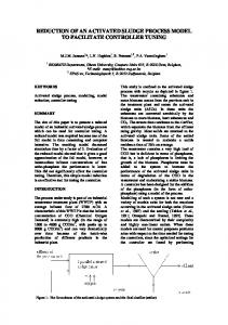
Return Activated Sludge Process Model
Aeration Tank Model
Adjustment of Oxygen intensity Mass balance
DO balance
Totalling the MLSS
Michaelis Menten Enzyme kinetics
Flow Balance
Growth rate adjustment
Totaly Mixed unit
Monod growth
Graphical interface
Constant input
Viable Biomass balance
Non Viable biomass balance
Final Clarifier Model
F.C. Graphical interface Areation tanks graphical interface
FC model test
Layer concentration
Settling velocity
substrate balance
Cascade (COD removal, nitrification and denitrification are alternating according the DO level)
Figure 1 Model tree diagram
Figure 2 Aeration tank graphical interface
Figure 3 Final clarifier graphical interface
MODEL IMPLEMENTATION
The previous formulation of the process model enables the model implementation using data driven programming. Thus, using a reasonable time step each variable can be calculated without the need to implement numerical solution routines. The results are very similar to solving the equation using the Euler numerical method. Equations from (1) through (17) are implemented on LabView, instrumentation-programming package, as virtual instruments (VIs). Thus, they can be linked to real instruments and actuators of the plant to function on-line. The model parameters can be tuned on-line. The process can be monitored on real time. Different control strategies can be tested and applied to either directly sensed variables or those calculated by the model. Figure (1) shows the hierarchical structure of the implementation. Three biological processes are considered: the COD removal, the nitrification and the denitrification. They are in a cascade structure. Each process will be activated according the DO level: (< 0.2) for denitrification in the anoxic zones, (> 0.2) for COD removal and (> 1) for nitrification to be activated. Figures 2 and 3 Water Intelligence Online August 2004 ©2004 The Authors
show user interfaces to the process units. Through one window, the plant operator can monitor the evolution of different components in the aeration tank by just pressing the appropriate buttons. The components are calculated by the model. The application can be easily extended to have some of the components measured on-line, validated and the correct value shown. The solids profile in the final clarifier is viewed and can be checked regularly by inspecting the final clarifier unit or compared to turbidity measurements. A friendly interface to the process controls was developed (not shown). The plant operator can act or adjust the set points manually and the results will be reflected directly on the other interfaces. Also, control actions can be automated in relation to the estimated/measured variables and just viewed through the interface. CONCLUSIONS
The presented model applies the principal kinetics of RAS biological reactions, mass balances each component, and empirically formulates major disturbances (temperature, dissolved salts and settleability characteristics). It is implemented on an instrumentation-programming package in a hierarchical modular structure. Different biological processes are sorted in cascade where they will be activated according the practical DO level. The modular structure and the use of instrumentation programming make the implementation easy to be extended and connected to sensors and actuators. Indeed, the implementation uses a friendly interface The model parameters can be estimated off-line. Different control strategies and operation scenarios can be studied. After tailoring the instrumentation and control equipment suitable to the plant, the model can be regularly checked and recalibrated as it is in use and continue for real time monitoring and control of the AS plant. REFERENCES Bailey J.E. and Ollis D.F. (1986) Biochmical Engineering Fundamentals, McGraw-Hill international Editions, NewYork. Catunda P. F. C. and Van Haandel A. C. (1992) Activated Sludge Settling Part I: Experimental determination of Activated Sludge Settleability, Water SA 18(3) 165-172. Jones G. L., (1973) Bacterial growth kinetics: Measurement and significance in the activated sludge process, Water Research 7, 1475-1492. Takacs I, Patry G. G., and Nolasco D. , (1991) A dynamic model of the clarification-thickening process, Water Research, 25(10) 1263-1271. Vanrolleghem P.A. and Lee D.S. (2003) On-line monitoring equipment for wastewater treatment processes: State of the art. Wat. Sci. Tech., 47(2), 1-34. Zaher U. E. (2000) Dynamic modeling of the return activated sludge process for real time monitoring and control, with special reference to: Gabal El-Asfar wastewater treatment plant- Msc. thesis, Cairo University-Faculty of Engineering, Giza, Cairo, Egypt. NOMENCLATURE µ(t) : bacterial growth rate (d-1) Ψ(t): rate of enzyme reaction (d-1) µmax : maximum specific growth rate (d-1) Ψmax: the maximum enzyme rate (d-1) C: mass balance parameter Ci: Influent concentration (mg/l) CR: Return concentration (mg/l) DO(t): current dissolved oxygen concentration (mg/l). DOC(t) :oxygenation intensity in mg O2 /min. Doin(t): DO concentration in the influent flow (mg/l). F(t): influent flow (m3). FR: return flow (m3) Kd: death rate (d-1). KDO: mg COD equivelent of mg mass of substrate.
Water Intelligence Online August 2004 ©2004 The Authors
Ko: half-saturation coefficient for Oxygen. Ks: half-saturation coefficient for substrate Mm: Oxygen required by endogenous respiration mgO2/g biomass. S: substrate concentration (mg/l). Sin: influent substrate concentration (mg/l). SSVI: stirred sludge volume index T: Temperature °C. V(t) : reactor volume (m3). Xnv: non viable bacteria concentration (mg/l). Xt : total bacterial cells concentration (mg/l). Xv: viable bacteria concentration (mg/l). Xv,in: influent viable bacteria (mg/l). Yx: the bacterial cells yield factor (mg/l). Z: Dissolved salts concentration (mg/l).