Nonlinear modeling of activated sludge process using the ...

E3S Web of Conferences 10 , 00119 (2016)

DOI: 10.1051/ e3sconf/20161000119

SEED 2016

Nonlinear modeling of activated sludge process using the HammersteinWiener structure Paweł Frącz 1,a 1

Opole University of Technology, ul. Prószk owsk a 76, 45-758 Opole, Poland

Abstract. The paper regards to physical model of the Activated Sludge Process, which is a part of the wastewater treatment. The aim of the study was to describe nitrogen transformation process and the demand of chemical fractions, involved in the ASP process. Moreover, the non-linear relationship between the flow of wastewater and the consumed electrical energy, used by the blowers, was determined. Such analyses are important from the economical and environmental point of view. Assuming that the total power does not change the blower is charging during a year an energy amount of approx. 613 MW. This illustrates in particular the scale of the demand for energy consumption in the biological aeration unit. The aim is to minimize the energy consumption through first building a model of ASP and then through optimization of the overall process by modifying chosen parameter in numerical simulations. In this paper example measurement and analysis results of nitrite and ammonium nitrogen concentrations in the aeration reactor and the active power consumed by blowers for the aeration process were presented. Further the ASP modeling procedure, which uses the Hammerstein-Wiener structure and example verification results were presented. Based on the achieved results it was stated that the developed set of methodologies may be used to improve and expand the overriding control system for system for wastewater treatment plant.

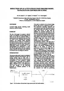
1 Introduction 1.1. The Activated Sludge Process The Activated Sludge Process (ASP) is a method used for biological wastewater treatment and is widely used in sewage treatment plants, for example [1]. Basic ASP process flow diagram is shown in Figure 1. The wastewater is brought into the biological reactor. The activation of wastewater process is based on providing oxygen to increase the number of microorganisms, responsible for contaminants reduction in the aeration tank. The activated sludge is then formed; it consists of flocks, mixes with new incoming wastewater and finally takes form of slurry. The flocks contain bacteria but also ciliates, flagellates, protozoa, nematodes, rotifers, larvae of insects, arachnids and mushrooms. Typical flock size varies from 50 µm to 100 µm. The sludge from the biological reactor is then transported to secondary settling tank (also called clarifier), in which the activated sludge is separated. A considerable part of the sludge is returned back to the reaction chamber (biological reactor) and the excessive part of the sludge is removed. The advantage of this method is its significant performance of harmful chemicals reduction. The main disadvantage is connected with high costs of electrical energy, which supply is needed for to assure a suitable amount of oxygen bowing into the aeration tank. Bacteria’s growth requires a continuous supply of energy. The heterotrophic bacteria require oxygen and organic a

carbon as a substrate. The autotrophic bacteria grow in oxygen environment using inorganic carbon substrate.

Figure 1. The basic principle of Activated Sludge Process.

1.2. Biological removal of nitrogen compounds Nitrogen is present in the wastewater in various forms, e.g. free form of ammonia, nitrates, nitrites, and different kinds of organic compounds. The total content of nitrogen is a sum of its particular components. Nitrogen is essential for biological growth, but in certain forms it is toxic and therefore, its reduction is desirable. Ammonia is toxic for aquatic organisms, among others, for fish. Nitrate presence causes excessive demand for oxygen. Nitrogen, as a nutrient, causes excessive growth of aquatic plants. There are two basic nitrogen transformation processes in the wastewater treatment plants: the nitrification and the denitrification. Both processes result in the removal of nitrogen from wastewater. Nitrification is the oxidation of ammonia and ammonium salts into nitrites and nitrates. This process is driven by nitrifying bacteria. Autotrophic nitrification takes place in the presence of oxygen at a concentration of at least 2 mg O2/dm3. Nitrification

Corresponding author: [email protected]

© The Authors, published by EDP Sciences. This is an open access article distributed under the terms of the Creative Commons Attribution License 4.0 (http://creativecommons.org/licenses/by/4.0/).


DOI: 10.1051/ e3sconf/20161000119

SEED 2016

others, TUDP model are described in [5-6]. The activated sludge system model is composed not only from the activated sludge (biochemical model, e.g. ASM), but also it includes models of other processes, in particular: he sedimentation model (settler model) and the mass transfer model (hydraulic model, aeration system model). Most of the simulation models, described in the literature, were carried out for the biological purification stage and thus the system consisted of the activated sludge reactor and the secondary sedimentation/settling tank [7]. The newest trends in modeling of wastewater treatment processes, however, seek to include also other system parts/processes, instead of only the specified area, in the multiphysical model. In such as a manner the whole wastewater treatment plant constitutes the object under study and the designed model includes additionally the sewage, sewage treatment plant and the receiver [8]. A factor impeding modeling of the technological sequence of the entire wastewater treatment plant lies in the fact that not all models of wastewater or sludge treatment processes have a common set of variables. For example one may consider a combination of the ASM1 model with a settler model. Such a hybrid model, however, involves the concentration of slurries from the settler as state variable, but this value is not present in the activate sludge process. This problem might be solved by using a complex variable, corresponding to the concentration calculated from the respective ASM1variables, which is, however, not a state variable. Another example of biochemical transformations model, which uses a different set of variables, is the ASM model and the methane fermentation - ADM1 (Anaerobic Digestion Model No.1) model. The most important part prior modeling is collection of measurement data, which allows the model to be accurately calibrated and validated for all conditions. The modern modeling approaches and algorithms are relatively easy to understand for engineering application purposes. They enable to model the wastewater treatment facilities and to calibrate them, which provide then accurate predictions of the system behavior under different operational conditions. Nowadays in every facility there are specialized measurement and SCADA devices installed for registering and collection of hydraulic and technological parameters. Given sufficient data, a modeler can accurately model the activated-sludge process using different models. Developments in the field of modeling of sludge treatment processes, including both dynamic and steadystate conditions, are well presented in [9]. Based on a literature review Author enhances the importance of computer modeling of activated-sludge process during design of new and optimization of existing wastewater plants. Readers who are interested in other interesting research results dealing with modeling of activated sludge tanks are referred [10-14]. In this paper chosen analysis result of nitrate and ammonium nitrogen and blower active power values, measured in experiments, are presented. Furthermore, the ASP modeling procedure and results of this model verification are described.

reaction consists of two phases. In the first stage bacteria oxidize ammonium to nitrite: + 1.5

→

+

+2

(1)

In the second stage nitrite ions are oxidized to nitrate by bacteria: + 0.5 → (2) The condition of autotrophic nitrification occurrence is, beside the oxygen presence, the presence of coal, as an energy source for autotrophic bacteria (e.g. carbon dioxide) and the appropriate pH value (around 7.5). Denitrification is a reduction of nitrite to nitrogen. This process takes place under anaerobic conditions. Oxygen is present in the nitrite. Bacteria use it instead of dissolved oxygen. A simplified description of the denitrification reaction is as follows: 2

+2

→

+

+ 2.5

(3)

1.3. Modeling of the Activated Sludge Process The practical aim of our work is to develop a set of methodologies that will be used to improve and expand the precedent control system for wastewater treatment plant. The overriding control system provides measurement data to the subordinating control systems of the plant and replaces in this way human service for sewage treatment plants. Conducted works aim to determine the nature of changes, dependencies, trends and to make other observations of the wastewater parameter values, which characterize the treatment process. The study uses empirically acquired and digitally processed data in order to identify develop and verify a non-linear simulation model of the wastewater treatment plant. The hypothesis relates to confirmation the possibility of use of a physical model of wastewater treatment plant, based on Hammerstein-Wiener structure, to optimize the treatment process. According to the latest global trends, mathematical modeling has become an integral part of the design and operation of wastewater treatment systems, particularly those using the ASP [2]. Simulation of the activated sludge systems (experiment carried out on the model) proved to be an extremely useful tool for operators, designers and consultants, as well as for the scientific community. The use of mathematical models allows one for to examine in a short time and with low financial outlay of many technological solutions, and for simulation of events from outside the range of typical real system conditions. The most common physical model is the ASM1 (Activated Sludge Model No.1), which was the first bio kinetic model of activated sludge. Implementations of the ASM1 in several popular simulation programs were compared in an exhaustive manner [3]. Examples of modified, supplemented or improved models of ASM1, known respectively as ASM2, ASM2d and ASM3 are described in detail in [1]. In addition to the ASM family models, in which the mass balance is based on the COD, there are also models that use the mass balance of the BOD, for example the ASAL models [4]. Models describing in detail the metabolism of organisms involved in the pollutants decomposition, which include, among

2


DOI: 10.1051/ e3sconf/20161000119

SEED 2016

2 Experimental results analysis

a stochastic component and significant own variances for time delays, which are multiples of 24h day.

2.1. Analysis results of nitrate nitrogen concentration Nitrate nitrogen NO3-N is next to nitrite nitrogen NO2-N the main product of decomposition of ammonium NH4-N. This value was registered during measurements by using an ion-selective probe from Hach-Lange. The measuring sensor was placed inside the oxygen reactor. Under normal operational conditions, the gathered data should indicate significantly lower values in the effluent as compared to these in the influent of the reactor.

Power density spectrum [dB]

50

-50

-100

10

-6

-4

10 Frequency [Hz]

10

-2

Figure 4. Power spectrum density calculated over the nitrate nitrogen concentration gathered during the measurement campaign.

12 10

3 x 10

=8 mg/dm 3

8

Autocovariance (mg/dm3) 2

Nitrate nitrogen concentration [ mg/dm3 ]

0

-150

14

6 4 2 0

2

4 time [d]

6

8

Figure 2. Time course of the nitrate nitrogen NO3-N concentration.

2

5

 = 24h 0

1 0 -1 -2 0

In Figure 2 example time course of the nitrate nitrogen measured within a week is presented. A periodical pattern can be recognized: the values are generally lower at night and higher at mornings. The nitrate nitrogen concentration varies in the range from 4 to 12.5 mg/dm3. The average value µ equals 8 mg/dm3.

50

100 Time delay [h]

150

Figure. 5. Autocovariance function calculated over the nitrate nitrogen concentration gathered during the measurement campaign.

Correspondent result was obtained by examining variation of the frequency structures over time, what is illustrated in Figure 6. The scale graph depicts no significant harmonics in the gathered data.

0.35 0.3 0.25

2

Energetic participation of wavelet coefficients 4 6 8 10 12 14

0.2 0.15 0.1

Scale (referred to 1h)

Probability density function [ ( mg/dm3 )-1 ]

(24h) -1

0.05 0 4

6 8 10 12 3 Nitrate nitrogen concentration [mg/dm ]

14

Figure 3. Probability density function calculated over the nitrate nitrogen concentration gathered during the measurement campaign.

In Figure 3 probability density function calculated over the nitrate nitrogen concentration gathered during the measurement campaign is presented. The probability density function depicts no uniform mode. Variability in the entire interval is relatively equal. In Figure 4 power spectrum density calculated over the nitrate nitrogen concentration gathered during the measurement campaign is presented. Power spectrum depicts several periodicity components of the sludge what is indicated by picks in the spectrum. The most significant value is the fundamental frequency component equal to 1*10e-5, the conversion of 24 hours. In Figure 5 the auto covariance function calculated over the nitrate nitrogen concentration gathered during the measurement campaign is presented. It indicates

39 36 33 30 27 24 21 18 15 12 9 6 3 0

x 10

1

2

3 4 Time [h]

5

6

-3

7

Figure 6. Scalegraph calculated over the nitrate nitrogen concentration gathered during the measurement campaign.

2.2. Analysis results of ammonia nitrogen concentration The concentration of ammonium nitrogen NH4-N was measured using two probes: the Hach-Lange and the Endress-Hauser sensors. Both sensors were placed inside the oxygen reactor. In Figure 7 time course of the ammonium nitrogen concentration measured with two different probes is presented. A periodical pattern can be recognized. But in contrast to the nitrate concentration, ammonium nitrogen indicates higher values

3


DOI: 10.1051/ e3sconf/20161000119

SEED 2016

20

is presented. The spectrum depicts periodicity of the sludge what is indicated by a pick near the 1*10e-5 frequency value. Certain importance is give also to the second harmonic component. In Figure 10 auto covariance function calculated over the ammonium nitrogen concentration gathered during the measurement campaign by the Hach-Lange probe. Here a high value of the covariance of time delay, which is equal to 24 h, and for the subsequent multiples, is depicted. 15 x 10 Autocovariance (mg/dm3) 2

Ammonium nitrogen concentration [ mg/dm3 ]

in the afternoons and at nights and lower at mornings. Values measured by the Hach-Lange probe were slightly lower as compared with data registered by the EndressHauser probe. The ammonia nitrogen concentration varies in the range from 0.8 to 19.5 mg/dm3. The average values µ=8 mg/dm3 for the Hach-Lange and µ=9 mg/dm3 for the Endress-Hauser probes. The standard deviation equals 4.09 for the Hach-Lange probe, and it is approx. 16% higher for the Endress-Hauser probe. In further studies the Hach-Lange probe was applied. Endress-Hauser probe Hach-Lange probe

15

10

 =9 mg/dm 3 1 =8 mg/dm 3 2

5

2

4 Time [d]

6

0

5

0

Scale (referred to 1h)

0.1

0.05

5 10 15 Ammonium nitrogen concentration [mg/dm 3 ]

Figure 8. Probability density function calculated over the ammonium nitrogen concentration gathered during the measurement campaign by the Hach-Lange probe. (24h)

-40 -60 -80 -6

1

2

3 4 5 6 7 Time [h] 0.005 0.01 0.015 Energetic participation of wavelet coefficients

2.3 Analysis results of the blower active power The next parameter analyzed was the active power applied for three different blowers that are installed in the reactor. The time courses for the various blowers are shown in Figure 12. The total value of blowers active power is presented in Figure 13. The average value of active power µ was equal to approx. 70 kW. Additional the probability density function was calculated over the active power values (Figure 14), which was approximated by using normal distribution function achieving very high fit (Pearson determination coefficient R2=0,89). Calculated standard deviation value depicts that during the entire measurement campaign the blowers have had relatively small active power, which was equal to 70 kW.

0 -20

10

39 36 33 30 27 24 21 18 15 12 9 6 3 0

Figure 11. Scalegraph calculated over the ammonium nitrogen concentration.

-1

20

-100

150

In Figure 11 scale graph calculated over the ammonium nitrogen concentration gathered during the measurement campaign by the Hach-Lange probe is presented. One can recognize similar periodic components as compared to the nitrate nitrogen concentration. For the entire duration of measurement the 24h daily component does not change its energy. Wavelet coefficients for the scale corresponding to the 1/(12h) frequency occur sporadically.

0.15

40

100 Time delay [h]

Figure 10. Autocovariance function calculated over the ammonium nitrogen concentration gathered during the measurement campaign by the Hach-Lange probe.

0.2

0 0

50

8

In Figure 8 probability density function calculated over the ammonium nitrogen concentration gathered during the measurement campaign by the Hach-Lange probe is presented. The highest probability occurred for the concentration equal to about 14 mg/dm3. The distribution has a fuzzy character and values are within the range from 0 to 16 mg/dm3. Probability density function [ ( mg/dm3 ) -1 ]

 = 24h

-5 0 0 0

Figure. 7. Time course of the ammonium nitrogen NH4-N concentration measured with two different probes.

Power density spectrum [dB]

10

5

-4

10 Frequency [Hz]

10

-2

Figure 9. Power spectrum density calculated over the ammonium nitrogen concentration gathered during the measurement campaign by the Hach-Lange probe.

In Figure 9 power spectrum density calculated over the ammonium nitrogen concentration gathered during the measurement campaign by the Hach-Lange probe

4


DOI: 10.1051/ e3sconf/20161000119

SEED 2016

for validation. Weekly measurement data were used for the modeling process. The available waveforms were divided in two half: one half - 3.5 day, was used for identification of the model, as the learning sequence (LS); the remaining 3.5 days was used for testing purposes, as a test sequence (TS). All data sets applied in the study consisted of 336 measuring points, i.e. 84 hours with four samples per hour. In a series of simulations an optimal nonlinearity on the input and output of the model were determined. Also an appropriate structure of the linear dynamic member was selected. For the estimation of non-linear members a piecewise-linear model was applied. Three different criteria for evaluation of the model quality were used: 1. C1: Best fit for learning sequence FIT(LS), 2. C2: Best fit for test sequence FIT(TS), 3. C3: Best fit for the sum over the learning and test sequences FIT(LS) + FIT(TS).

The momentary power reaches the maximum value of 120 kW. Activ power PD1

100 50 Activ power [kW]

0 0

2

4 Activ power PD2

6

8

2

4 Activ power PD3

6

8

2

4 Time (days)

6

8

0.06 0.04 0.02 0 50 0 0

Figure 12. Time course of the active power applied for particular blowers. 140

3.1. Non-linear process identification of nitrate nitrogen SNO production in the aerobic reactor In the first step the model for nitrate nitrogen (SNO) was identified and verified. The input of the SISO model was the outflow of sewage. The output variable was the course of SNO. The sampling period for both variables was 15 min. Both variables were changing over time. A genetic algorithm was used for to determine five parameter values, which were as follows:  number of zeros (plus 1) – P1,  number of poles – P2,  input delay – P3,  number of piecewise-linear estimators of the input nonlinearity (plus 1) – P4,  number of piecewise-linear estimators of the output non-linearity (plus 1) – P5. For model goodness indication, the following equation was applied:

100

D1

D2

D3

Total activ power P +P +P [kW]

120

80

=70 kW

60 40 20 0

2

4 Time [d]

6

8

Figure 13. Time course of the total blower active power.

Assuming that the total power does not change during the year blowers charge an energy amount of approx. 613 MW. This illustrates in particular the scale of the demand for energy consumption in the biological aeration unit. Probability density function Activ power [kW-1 ]

0.1

P

D1

+P +P , N(=70,=7), R2 =0.8912 D2

D3

0.08 0.06

= 100 ⋅ 1 −

0.04

40

60

80 Time [d]

100

120

140

Figure 14. Probability density function calculated over the active power values. The solid line corresponds to approximation estimated by means of normal distribution.

3 Non-linear modeling of processes involved in the ASP

) ̅)

[%]

(4)

Where: Y is the model response, C is the measured data. This value is given in percent, therefore the higher the result, the better the fit. The summary results of studies, which aimed determination of the best structure for the different criteria analyzed, are listed in Table 1. All the structures were found to have the same number of zeros P1=3, the same number poles P2=7 in the dynamic part and the same delay, which was equal to one step P3=1. Differences were calculated for the number of piecewise-linear estimators of the input and output nonlinearities.

0.02 0 20

( (

chosen

The study was carried out to identify certain processes related to waste water treatment. The purpose of these studies is an alternative description of the treatment of nitrogen and chemical fractions of demand. Moreover, the aim of research is to determine the non-linear relation between the flow of sewage and electric energy consumed. The process is treated as a Single Input Single Output (SISO). The identification was carried out using Hammerstein-Wiener model. The study was conducted using MATLAB Toolbox System Identification Toolbox. In the studies two sets of data were applied: one for identification and one

Table 1. Comparison of the best fit Hammerstein-Wiener structures found for the three considered criteria; output – the nitrate nitrogen SNO concentration, input – sludge flow.

5

Crit.

P1

P2

P3

P4

P5

C1

3

7

1

4

4

FIT(LS ) [%] 87.55

C2

3

7

1

3

2

78.33

76.19

C3

3

7

1

1

3

83.48

74.80

FIT(TS) [%] 68.27


DOI: 10.1051/ e3sconf/20161000119

SEED 2016

of zeros P1=7 and poles P2=7. It had respectively 2 (P4) and 6 (P5) points of inflection of the input and output nonlinearity estimators. It was found that criteria C2 and C3 meet the same structure with two zeros and three poles in the dynamic part. The static nonlinearity input estimator had 6 piecewise-linear (P5=5+1), while the output nonlinearity estimator included four piecewise-linear.

When used as criterion the best fit of learning sequence (no. 1), the optimal structure consisted of 5 piecewiselinear (P4x=4+1)in both nonlinearity estimators. An example time course of nitrate nitrogen model identified using the learning sequence is shown in Figure 15. The model relatively properly reproduces the measured nitrate nitrogen values adjusting to changes in the following days. Negligible mismatches occur only at the hourly/minutely variability level of the data. Nitrate nitrogen concentration [mg/dm3 ]

14

Table 2. Comparison of the best fit Hammerstein-Wiener structures found for the three considered criteria; output – the ammonium nitrogen concentration N-NH4, input – sludge flow.

Measurement SNO (LS) Simulation FIT=87.5579

Crit.

P1

P2

P3

P4

P5

FIT(LS) [%]

FIT(TS) [%]

10

C1

7

7

1

2

6

85.46

55.69

8

C2

2

3

1

5

3

81.18

62.17

C3

2

3

1

5

3

81.18

62.17

12

6 4 0

0.5

1

1.5 2 Time [days]

2.5

3

An example time course of ammonium nitrogen model identified using the LS is shown in Figure 17. The residuals (Figure 18) are in the range of from -2.7 to 1.5 mg/dm3. Stochastic nature of the residuals time course confirms that the model has been selected properly.

3.5

Ammonium nitrogen concentration [mg/dm3]

Figure 15. Timing charts of the Hammerstein-Wiener model in response to nitrate nitrogen data contained in the LS (first 84 hours); Identification according to the criterion C1.

1

0.5

0

-0.5

-1 0

Measurement N-NH4 (LS) Simulation FIT=81.183

12 10 8 6 4 2 0 0

0.5

1

1.5 2 Time [days]

2.5

3

3.5

Figure 17. Time course of the Hammerstein-Wiener model in response to ammonium nitrogen data contained in the LS (first 84 hours); Identification according to the criterion C3. The residues of training sequence LS [mg/dm3]

The residues of training sequence LS [mg/dm3]

The residuals time course of the Hammerstein-Wiener model in response to learning sequence, when identification considered the criterion C1, is presented in Figure 16. The values are in the range from -0.8 to 1mg/dm3.The stochastic nature of the residuals within time course, confirms that the model has been selected properly.

14

0.5

1

1.5 2 Time [days]

2.5

3

3.5

Figure 16. The residuals of the Hammerstein-Wiener model in response to LS; Identification according to the criterion C1.

3.2. Non-linear process identification of ammonium nitrogen NH4-N production in the aerobic reactor We then consider the process, in which the wastewater outflow was given as the input of the SISO system, and the discharged ammonium nitrogen concentration (NH4-N) was assumed as output. The sampling period for both datasets was equal to 15 min. Just as for the nitrate nitrogen identification, during these studies it were used two datasets: one for the identification and second for the validation. Also the same genetic algorithm, the same number of parameters of the objective function, the same goodness indicator and the same criteria were applied. The summary of the results obtained are listed in Table 2. The optimal model structure, for which the best matching value was calculated, occurred for identification with the LS (criterion C1). It had a significant number

2 1 0 -1 -2 -3 0

0.5

1

1.5 2 Time [days]

2.5

3

3.5


3.3. Non-linear process identification of active power AP used for in the aeration Then, an attempt to determine the non-linear relationship between the amount of effluent and environmental parameters: temperature, pressure and active power consumption was made. The model inputs were: sludge outflow, with sampling period equal to 15 min, temperature and pressure, with sampling period equal to 60 min. The model output was the total active power, which constitutes the sum of active power values measured on three blower devices mounted for aeration in the

6


DOI: 10.1051/ e3sconf/20161000119

SEED 2016

biological reactor. All datasets were interpolated in order to obtain a uniform sampling rate (1/4 h -15 min). As in the previous studies, two sets of data, 84 hours measuring period, were used for the model identification and validation. A genetic algorithm was used for to determine 11 variables: P1 for sewage outflow: P1S, P1 for Temperature: P1T, P1 for Pressure: P1P, P2 for sewage outflow: P2S, P2 for Temperature: P2T, P2 for Pressure: P2P, P3 for sewage outflow: P3S, P3 for Temperature: P3T, P3 for Pressure: P3P, P4 and P5. For estimation of model goodness eq. (4) was applied. Three different criteria were used for evaluation of the model quality, when checking for the best fit within the learning, testing and the total sum of this both values. The final results of studies aiming determination of the best structure for the different criteria are listed in Table 3. The best fitted structure was meet for the learning sequence (criterion C1).

The residues for LS [kW]

10

P1

P2

P3

P4

P5

FIT(LS) [%]

FIT(TS) [%]

C1

3

2

1

2

1

12

1

C2

3

2

1

2

1

12

2

C3

3

1

1

2

2

12

3

Total active power [kW]

80 70 60 0.5

1

1.5 2 Time [days]

2.5

3

-15 0.5

1

1.5 2 Time [days]

2.5

3

3.5

Modeling results of three selected processes occurring in the aeration reactor of wastewater treatment plant are presented in this paper. The Hammerstein-Wiener structure was applied for identification of the process of nitrate nitrogen SNO production, the process of ammonium nitrogen N-NH4production and the process of active power supply AP during aeration. For each of the models identified three criteria were applied: C1: Best fit for the learning sequence FIT(LS), C2: Best fit for the test sequence FIT(TS), C3: Best fit for the sum of the learning and test sequences FIT (LS)+FIT(TS). Analysis of the results allowed for to define the following conclusions: 1. All the models received reproduce relatively correctly the actual measurements. The best fit for the SNO model was found using the criterion C1 for the LS, which was equal to 87.55%. The best fit for the N-NH4 model was found for the criterion C1 for the LS, which was equal to 85.46%. The best fit for the AP model was found by using the criterion C1 within the LS, and which equaled 87.55%. The best fit for the TS was obtained for criterion C2, for all identified models. 2. Residuals were differently for each of the models. For criterion C1, residuals were stochastic and were not correlated with the time courses, by which it can be concluded that the chosen models are appropriate. For other criteria residual values ranged from -4 to 5 mg/dm3 for both nitrogen models and from -15 to +12 kW for the active power model. 3. The achieved results confirmed the hypothesis that it is possible to use a physical model of the ASP based on Hammerstein-Wiener structure for to optimize the wastewater treatment process.

90

50 0

-10

4 Conclusions

Measurement (LS) Simulation FIT=65.4621

100

-5


An example time course of active power model identified using the test sequence is shown in Figure 19. The model relatively correctly provides the active power values when based on the given input data. The residuals (Figure 20) are in the range of from -8 to 10 kW. They indicate a single error in the measurement data around the 50th hour of measurement. 110

0

-20 0

Table 3. Comparison of the best fit Hammerstein-Wiener structures found for the three considered criteria; output –the active power consumed by the blower. Crit.

5

3.5

Figure 19. Timing charts of the Hammerstein-Wiener model in response to active power data contained in the LS (first 84 hours); Identification according to the criterion C2.

References

Summing up the results it is to conclude that the developed ASP process model using the HammersteinWiener structure allows conducting simulation studies, which concern determination of the amount of energy consumption. The electrical energy is used by the blower in the aerobic reactor of a wastewater treatment plant for aeration. Presented results confirm the efficacy of the developed methodology for application to carry out simulation studies aimed at optimization of the ASP process.

1. G. Bitton, Wastewater Microbiology, 3rd edition, Chapter 8. Activated Sludge Process 2. M. Henze, W. Gujer, T. Mino, M. van Loosdrecht, IWA Scientific and Technical Report No. 9, IWA Publishing. London, UK (2000) 3. J. B. Copp, Office for Official Publications of the European Community, Luxembourg. ISBN 92-8941658-0 4. A. J. Stokes, J. R. West, C. F. Forster, W. J. Davis, Water Res., 34 (4), 1296-1306 (2000)

7


DOI: 10.1051/ e3sconf/20161000119

SEED 2016

5. E. Murnleitner, T. Kuba, M. C. van Loosdrecht, J. J. Heijnen, Biotechnol. Bioeng. 54, 434-450 (1997) 6. H. M. van Veldhuizen, M. C. van Loosdrecht, J. J. Heijnen, Water Res., 33, 3459-3468 (1999) 7. J. Makinia, M. Świnarski, E. Dobiegala, Wat. Sci. Techn., 45 (6), 209-218 (2002) 8. W. Gujer, Wat. Sci. Tech., 53 (3), 111-119 (2006) 9. M. Smith, J. Dudley, Wat. & Envir. J., 12 (5), 346-356 (1998) 10. Z. Lin, S. Lu, Wat & Envir. J., 25, 573-587 (2011) 11. S. Plessis, R. Tzoneva, Water SA, 38 (2), 287-306 (2012) 12. Z. Sadecka, A. Jędrczak, E. Płuciennik-Koropczuk, S. Myszograj and M. Suchowska-Kisielewicz, Chem. Biochem. Eng. Q., 27 (2), 185-195 (2013) 13. C. Fall, E. Millán-Lagunas, K. M. Bâ, I. GallegoAlarcón, D. García-Pulido, C. Díaz-Delgado, C. SolísMorelos, J. Environ. Manage, 113, 71-77 (2012) 14. H. Boursier, F. Béline., E. Paul, Bioresource Technol., 96 (3), 351-358 (2002)

8