1692
JOURNAL OF THE ATMOSPHERIC SCIENCES
VOLUME 65
Dynamic Models for the Subgrid-Scale Mixing of Reactants in Atmospheric Turbulent Reacting Flows JEAN-FRANÇOIS VINUESA
AND
FERNANDO PORTÉ-AGEL
Saint Anthony Falls Laboratory, and Department of Civil Engineering, University of Minnesota, Minneapolis, Minnesota (Manuscript received 4 January 2007, in final form 14 August 2007) ABSTRACT The effects of the subgrid scales on chemical transformations in large-eddy simulations of the convective atmospheric boundary layer (CBL) are investigated. Dynamic similarity subgrid-scale models are formulated and used to calculate the subgrid-scale covariance. The dynamic procedure allows for simulations free of parameter tuning since the model coefficients are computed based on the resolved reactant concentrations. A scale-dependent procedure is proposed that allows relaxing the assumption of scale invariance used in the dynamic similarity model. Simulation results show that both models are able to account in part for the effect of the segregation of the scalars at the subgrid scales, considerably reducing the resolution dependence of the results found when no subgrid covariance model is used. The scale-dependent dynamic version yields better results than its scale-invariant counterpart.
1. Introduction Understanding and modeling chemical transformations in the atmospheric boundary layer (ABL) is complicated by the influence of physical processes, particularly turbulence, on the distribution and mixing of reacting scalars. The ability of turbulence to bring together and mix the reactants can have a strong influence on the chemical composition of the ABL. This influence is larger for relatively fast chemical transformations, for which the temporal scale of the chemistry is smaller than the characteristic temporal scales associated with the turbulence. Alternatively, chemical compounds with a low reactivity are typically well mixed throughout the ABL and, consequently, turbulent mixing has little influence on their reaction rates and concentration levels. Large-eddy simulation (LES) is a useful tool to study the effect of turbulence on chemistry in the ABL. Past studies have been mostly restricted to moderately fastreacting flows involving a second-order reaction between a pollutant emitted at the surface and one entrained from the free troposphere (Gao and Wesely
Corresponding author address: J.-F. Vinuesa, European Commission–DG Joint Research Centre, Institute for Environment and Sustainability, Ispra 21020, Italy. E-mail:
[email protected] DOI: 10.1175/2007JAS2392.1 © 2008 American Meteorological Society
1994; Molemaker and Vilà-Guerau de Arellano 1998; Patton et al. 2001; Petersen et al. 1999; Petersen and Holtslag 1999; Petersen 2000; Schumann 1989; Sykes et al. 1994; Verver et al. 1997; Vilà-Guerau de Arellano and Cuijpers 2000; Vinuesa and Vilà-Guerau de Arellano 2003). In these studies, it is assumed that chemical species are perfectly mixed within the grid volume of the LES and, consequently, there is no need to account for the subgrid-scale (SGS) reactant covariance. In addition, the effect of the chemistry on the subgrid-scale fluxes of the reactants is ignored and those fluxes are modeled using the same models and model parameters that are used for other nonreacting scalars. Krol et al. (2000) and Vinuesa and Vilà-Guerau de Arellano (2005) reported that for some reactants, such as OH in the reactions with hydrocarbons and with NO2, the assumption of homogeneous mixing at subgrid scales may not be always satisfied. When studying the dispersion of a reactive plume, Meeder and Nieuwstadt (2000) showed the importance of the segregation between reactants at the subgrid scales. More recently, Vinuesa and Porté-Agel (2005, hereafter VP05) showed that neglecting the subgrid-scale chemical transformations can lead to an overestimation of the reactivity of species involved in a second-order reaction. Therefore, in simulations of complex chemical mechanisms containing fast reacting scalars, LES may require a subgrid-scale model for the subgrid reactant
MAY 2008
1693
VINUESA AND PORTÉ-AGEL
covariance, that is, the quantity that accounts for the reactant mixing at the subgrid scales. In an effort to do that, Meeder and Nieuwstadt (2000) proposed to solve a budget equation for the subgrid covariance. Their formulation includes an eddy diffusivity subgrid flux model and closure models for third-order moments. A different approach, proposed by VP05, consists of using scale-similarity arguments together with a dynamic procedure to develop a tuning-free subgrid-scale model for the scalar covariance. The dynamic similarity model was shown to substantially improve the simulation results compared with the case without the subgrid covariance model. However, the results also revealed some scale dependence of the dynamically computed coefficient, which is in contradiction with the scale invariance assumption on which the dynamic model relies. In this paper, we develop a scale-dependent dynamic model for the reactant covariance by relaxing the scale invariance assumption used by VP05. The model is applied in simulations of an atmospheric boundary layer flow with two reactants involved in a second-order irreversible reaction (A ⫹ B → products). Emphasis is placed on the ability of the new model to capture the different effects of nonhomogeneous reactant mixing on the reaction rates associated with different scales (grid resolution).
By assuming scale similarity between resolved and subgrid scales, the subgrid covariance can be modeled as proportional to the resolved covariance at larger scales (typically between ⌬ and 2⌬). The subgrid covariance can then be expressed as ⌬ ˜B ˜ ⫺A ˜B ˜ 兲, ⫽ C sim 共A
where the overbar represents spatial filtering at scale 2⌬ and C ⌬sim is the similarity coefficient. Since this coefficient may depend on the chemical regime, and to avoid tuning or a priori specification, it is evaluated directly from the resolved scales by using a dynamic procedure (VP05). For the scalar covariance, the dynamic procedure is based on the Germano identity (Germano et al. 1991): ˜B ˜ ⫺A ˜ B ˜, ϒ⫽⌶⫺⫽A
冉
共1兲
˜ is the spatially filtered (at scale ⌬) concentrawhere A tion of the reactant A, which reacts following the second-order irreversible reaction k
共2兲
The effect of the unresolved scales on the evolution of the filtered scalar concentration appears through the subgrid-scale flux QA,i and the subgrid-scale reactant covariance . The SGS flux is defined as ⬃ ˜, QA,i ⫽ ui A ⫺ u˜i A
共3兲
and the SGS reactant covariance that accounts for the mixing of the reactant at subgrid scales is ⬃ ˜B ˜. ⫽ AB ⫺ A
冊
^ ^^ 2⌬ ˜ B ˜ ⫺A ˜ B ˜ , ⌶ ⫽ C sim A
共7兲
where the caret represents a spatial filtering operation applied at scale 4⌬. Substitution of (5) and (6) into (7) leads to ⌬ X, ϒ ⫽ C sim
In large-eddy simulation, the filtered conservation equation for a reacting scalar involved in a secondorder reaction is
A ⫹ B → products.
共6兲
where ϒ is a resolved covariance that can be deter⬃ ˜ B ˜ is mined using the resolved scales and ⌶ ⫽ AB ⫺ A the subgrid covariance at a test-filter scale (2⌬). Using the similarity model, ⌶ can be expressed as
2. Subgrid-scale chemical transformations
˜ ˜ ⭸A ⭸QA,i ⭸A ˜B ˜ ⫹ 兲, ⫽⫺ ⫺ k共A ⫹ u˜i ⭸t ⭸xi ⭸xi
共5兲
共4兲
where, for ⌬ ⫽ 2⌬, X⫽
冉
冊 冉
共8兲
冊
2⌬ ^ ^^ C sim ˜ B ˜ ⫺A ˜ B ˜ ⫺ A ˜B ˜ ⫺A ˜B ˜ . A ⌬ C sim
共9兲
It is important to note that the original dynamic model assumes scale invariance of the model coefficient at the filter and test-filter scales; that is, ⌬ 2⌬ ⫽ C sim ⫽ Csim. C sim
共10兲
Minimizing the error associated with the use of the similarity model in (6) over all three vector components as well as over some direction of statistical homogeneity or over fluid pathlines (Meneveau et al. 1996) results in ⌬ ⫽ C sim
具ϒX典 . 具XX典
共11兲
In simulations of a simple second-order reaction in a convective boundary layer (CBL), VP05 showed that the dynamic similarity model substantially improved the simulation results compared with the case without subgrid covariance model. However, their results also
1694
JOURNAL OF THE ATMOSPHERIC SCIENCES
revealed some scale dependence of the dynamically computed coefficient, which is in contradiction with the scale invariance assumption on which the dynamic model relies. Next, a scale-dependent version of the dynamic similarity model for the reactant covariance is developed. The new model is inspired in the modeling approach previously developed for the dynamic Smagorinsky model for the SGS stresses (Porté-Agel et al. 2000) and for the eddy diffusivity model for the SGS inert scalar fluxes (Porté-Agel 2004). ⌬ Without assuming that C 2⌬ sim ⫽ C sim, we can still apply the dynamic model given by (11), (8), and (9). Note that ⌬ this change introduces a new unknown  ⬅ C 2⌬ sim/C sim. For scale-invariant situations,  ⫽ 1. To compute C ⌬sim using (11) one needs to estimate . A dynamic value for  can be obtained using a second test filter at scale ⌬ˆ ⬎ ⌬. For simplicity, and without loss of generality, we take ⌬ˆ ⫽ 4⌬, and denote variables filtered at scale 4⌬ by a caret (^). Writing the Germano identity between scales ⌬ and 4⌬ yields ⌬ ϒ⬘ ⫽ C sim X ⬘,
between scales ⌬ and 4⌬. A consequence of the as⌬ 4⌬ 2⌬ sumed local power law is that C 2⌬ sim/C sim ⫽ C sim/C sim ⫽ 4⌬ ⌬ 2 , and thus ␥ ⫽ C sim/C sim ⫽  . With this substitution, (16) only contains the unknown  and can be rewritten as a fifth-order polynomial on , P共兲 ⫽ A0 ⫹ A1 ⫹ A22 ⫹ A33 ⫹ A44 ⫹ A55 ⫽ 0. 共17兲 The coefficients Ai can be calculated as
X⬘ ⫽
冋 冉 4⌬ C sim
⌬ C sim
冊 冉
共13兲 c1 ⫽
冊册
== ^ ^ ^ ^ ^ ^ ^ ^ ˜ ˜ ˜B ˜ ⫺ A ˜B ˜ ⫺A ˜B ˜ AB ⫺ A ,
具ϒ⬘X ⬘典 . 具X ⬘X ⬘典
共15兲
共16兲
⌬ 4⌬ which has two unknowns,  ⫽ C 2⌬ sim/C sim and ␥ ⫽ C sim/ ⌬ C sim. To close the system, a relationship between  and ␥ is required. Thus, a functional form of the scale dependence of the coefficient needs to be postulated. As in Porté-Agel et al. (2000), we assume a power law of the form C ⌬sim ⬃ ⌬␣. For such a power-law behavior,  does not depend on scale and is equal to  ⫽ 2. Note that this assumption is much weaker than the standard dynamic model, which corresponds to the special case ⫽ 0. We stress that one does not need to assume the power law to hold over a wide range of scales, but only
共19兲
A2 ⫽ a1d2 ⫺ c2b1 ⫺ a2e1,
共20兲
A3 ⫽ c1d2 ⫺ c2d1,
共21兲
A4 ⫽ a1e2 ⫺ c2e1,
共22兲
A5 ⫽ c1e2,
共23兲
e1 ⫽
兲典,
冊冔
共24兲
2
˜B ˜ ⫺A ˜B ˜ A
冓冉 冓冉 冓冉
共25兲
,
冊冔 冊冉 冊冔
^ ^^ ˜B ˜ ⫺A ˜ B ˜ ϒ A
˜B ˜ ⫺A ˜B ˜ A
^ ^^ ˜B ˜ ⫺A ˜ B ˜ A
共26兲
,
^ ^^ ˜B ˜ ⫺A ˜ B ˜ A
冊冔
,
2
,
共27兲 共28兲
and
冓 冉
冊冔
^ ^ ^ ^ ˜B ˜ ⫺A ˜B ˜ a2 ⫽ ⫺ ϒ⬘ A , b2 ⫽
Setting (11) equal to (15) yields
具ϒX典具X ⬘X ⬘典 ⫺ 具ϒ⬘X ⬘典具XX典 ⫽ 0,
冓冉
d1 ⫽ ⫺2 (14)
⌬ ⫽ C sim
A1 ⫽ c1b2 ⫺ a2d1,
具共
b1 ⫽
where the overbrace ( ) denotes spatial filtering at scale 8⌬. Again minimizing the error as yields, besides (11), another equation for C ⌬sim is
共18兲
˜B ˜ ⫺A ˜B ˜ a1 ⫽ ⫺ ϒ A
where
and
A0 ⫽ a1b2 ⫺ a2b1,
where
共12兲
^ ^ ^ ˜B ˜ ˜B ˜ ⫺A ϒ⬘ ⫽ A
VOLUME 65
^ ^ ˜B ˜ ⫺A ˜B ˜ 冊 冔, 冓 冉A^ ^2
== ^ ^ ^ ^ ˜ ˜ ˜B ˜ c2 ⫽ ϒ⬘ AB ⫺ A
冊 冔, 冓 冉 ^ == ^ ^ ^ ^ ^ ^ ^ ˜ ˜ ˜ ˜ ˜ ˜ ˜B ˜ 冊 冔, d ⫽ ⫺2 冓 冉 AB ⫺ AB 冊冉 AB ⫺ A 2
==
e2 ⫽
冓 冉A^˜ B^˜ ⫺ A^˜ B^˜ 冊 冔. 2
共29兲 共30兲
共31兲 共32兲
共33兲
A Newton–Raphson method is used to find that root. Once  has been computed, it is used in (9) to compute X, which in turn is used in (11) to obtain C ⌬sim. The
MAY 2008
1695
VINUESA AND PORTÉ-AGEL
subgrid-scale reactant covariance is then calculated from (5) and used to obtain the total chemical term as shown in (1).
3. Numerical setup The simulations were carried out using the modified version of the LES code described by Albertson and Parlange (1999), Porté-Agel et al. (2000), and PortéAgel (2004). The main features of this code are as follows: • Filtered Navier–Stokes equations written in rota-
tional form are solved (Canuto et al. 1988).
of 2 ppb both in the CBL and in the free troposphere. The rate coefficient k is set at 2.1 ⫻ 10⫺2 ppb⫺1 s⫺1. The reaction rate coefficient and species concentrations are on the same order of magnitude as those found in the ABL (Krol et al. 2000). Turbulent reacting flows are commonly classified using two Damköhler numbers: (i) the turbulent Damköhler number, Dat, which refers to the influence of the largest atmospheric boundary layer eddies on the reacting scalars; and (ii) the Kolmogorov Damköhler number, Dak, that quantifies the relative effect of the smallest ABL eddies on the chemical transformations. For a reactant A involved in the second-order irreversible reaction (2), these numbers are calculated using
• Derivatives in the horizontal directions are computed
• • • •
•
using the Fourier collocation method, while vertical derivatives are approximated with second-order central differences (Canuto et al. 1988). Dealiasing of the nonlinear terms in Fourier space is done using the 3/2 rule (Canuto et al. 1988). An explicit second-order Adams–Bashforth time advancement scheme is used (Canuto et al. 1988). A two-step time advancement scheme for the chemical solver is used (Verwer 1994). Scale-dependent dynamic models for SGS stresses (Porté-Agel et al. 2000) and SGS scalar fluxes (PortéAgel 2004) are applied separately to each of the scalars (temperature as well as reacting scalars). A stress/flux-free upper boundary condition, a Monin– Obukhov similarity–based lower boundary condition, and a periodic lateral boundary condition are used.
We simulate the same dry convective atmospheric boundary layer described by VP05. A uniform sensible heat flux of 0.05 K m s⫺1 is prescribed at the surface. The initial potential temperature has a constant value of 311 K throughout the boundary layer, with an overlying inversion of strength 0.006 K m⫺1 above 700 m. The size of the computational domain is (2Lz, 2Lz, Lz) with Lz ⫽ 1500 m and it is divided into N ⫻ N ⫻ N uniformly spaced grid points. Three resolutions are used, corresponding to N equal to 48, 96, and 192. The maximum time step used in the calculation is 0.25 s and the simulations cover a 1-h period. The results presented below are obtained by averaging over the second half-hour. The corresponding convective velocity scale w and the friction velocity u are equal to 1.08 * * and 0.3 m s⫺1, respectively. We define a chemical setup based on the secondorder irreversible reaction given by (2). The reactant A is uniformly emitted at the surface with a flux of 0.25 ppb m s⫺1 and zero initial concentrations in the CBL; B is not emitted and its initial profile has a constant value
Dat,A ⫽
t , c
共34兲
Dak,A ⫽
k , c
共35兲
where t , k , and c are the turbulent, Kolmogorov, and the chemical time scales, respectively. In the context of LES, where only eddy motions smaller than the filter size (on the order of the grid size) are parameterized, it is of interest to use another nondimensional parameter, the subgrid Damköhler number, Dasgs (Krol et al. 2000; Molemaker and VilàGuerau de Arellano 1998; Vinuesa et al. 2006). This number is equal to the ratio between the characteristic time scale associated with the smallest resolved eddy motions sgs and the chemical time scale c; it reads Dasgs,A ⫽
冉 冊
sgs sgs ⫽ c ⑀sgs
1Ⲑ2
˜, kB
共36兲
where sgs and ⑀sgs are the subgrid-scale eddy viscosity and subgrid-scale dissipation rate of turbulent kinetic energy, respectively. The subgrid-scale dissipation rate is defined as the rate of transfer of kinetic energy between the resolved and the subgrid scales (Meneveau and Katz 2000; Pope 2000). In LES with a Smagorinsky eddy viscosity model, these quantities can be locally calculated as
sgs ⫽ C 2s ⌬2 | S˜ |
共37兲
⑀sgs ⫽ ⫺˜ ij S˜ ij ,
共38兲
and
where ˜ ij and | S˜ | are the subgrid-scale stress tensor and the magnitude of the resolved strain rate, respectively. By using Dasgs, the turbulent reacting flow can be classified with respect to the effect of the unresolved
1696
JOURNAL OF THE ATMOSPHERIC SCIENCES
VOLUME 65
TABLE 1. Mixed layer averaged subgrid Damköhler numbers. Scalar
483
963
1923
A B
1.66 0.02
0.96 0.02
0.56 0.02
scales on the chemistry. For Dasgs ⬍ 1, the flow is well mixed at the subgrid scale and, therefore, the unresolved scales do not influence the chemical transformation. For Dasgs ⬃ O(1) and larger, the reactants are not well mixed at the subgrid scales, which can result in a reduction or enhancement of the chemical transformations at those scales. Since the focus of this study is the effect of the unresolved scales on the chemical transformation and B shows Dasgs K 1 (see Table 1), the following analysis is restricted to the bottom-up scalar A.
4. Results Figure 1 shows the vertical profiles of the mean concentration of the reactant A for the three different resolutions (483, 963, and 1923) and the three different models for the subgrid-scale covariance (no model, i.e., ⫽ 0, the dynamic similarity model, and the scaledependent dynamic similarity model). The fact that the profiles obtained with the higher-resolution simulations do not change with the use of the subgrid-scale model highlights that the impact of the subgrid-scale covariance is very small and practically negligible at this resolution. For the lower resolutions, profiles obtained when no model is used for the SGS covariance in the chemical term (i.e., ⫽ 0) show important differences. The largest are found for the 483 simulation, in particular close to the surface. These underestimations are due to a faster depletion of A by reaction with B. The bulk Dasgs are larger than one for the lower resolution, ⬃O(1) for the 963, and lower than one for the higher resolution. For the lowest resolutions, segregation of the reactants at the subgrid scales is expected to affect the concentration. The reactants are not uniformly mixed at the subgrid scales and, consequently, the assumption of perfect mixing at those scales is not valid. In these cases, the chemical term in the concentration-governing equation that only includes resolved concentrations and not the subgrid covariance accounting for the heterogeneous subgrid mixing, that is, ⫽ 0 in (1), is overestimated. Since the depletion rate of the reactant A is overestimated, the concentration of A is underestimated. This is in qualitative agreement with the results shown in Fig. 1. The agreement with the 1923 experiments is largely
FIG. 1. Vertical profiles of dimensionless bottom-up reactant concentration for the (a) 483-gridpoint setup and (b) 963-gridpoint setup. Different models for the subgrid-scale covariance are used: no model, that is, ⫽ 0 (squares), the dynamic similarity model (triangles), and the scale-dependent dynamic similarity model (diamonds). The results obtained for the 1923 simulations are also shown using lines (the styles used, i.e., solid, dotted, and dashed lines, correspond to the different formulations, i.e., no model, dynamic similarity model, and the scale-dependent dynamic similarity model, respectively).
MAY 2008
1697
VINUESA AND PORTÉ-AGEL
FIG. 2. Vertical profiles of the similarity coefficients calculated dynamically by the scale-dependent procedure. The 483-, 963-, and 1923-gridpoint setups are represented by diamonds, triangles, and a solid line, respectively.
improved by using the similarity models. It is clear that by including a model for the nonhomogeneous mixing at the subgrid scales, LES is able to incorporate, at least partially, the effect of the unresolved scales on the chemical transformations. Moreover, accounting for scale dependence in the dynamic model further improves the results. However, despite these improvements, some differences between the numerical experiments are still noticeable close to the surface. Figure 2 shows vertical profiles of the similarity coefficients C ⌬sim calculated using the scale-dependent dynamic procedure. The scale-dependent dynamic coefficients are consistently larger than those obtained from the scale-invariant similarity model (see Fig. 2 in VP05). These trends in the coefficient, increasing with decreasing resolution, are expected to increase the subgrid-scale covariance and, as a consequence, reduce the depletion rate of the reactant A. This, in turn, yields higher concentrations of the reactant, which is consistent with the concentration results presented in Fig. 1. Notice that the grid resolution dependence of  appears to indicate a breakdown of the power-law assumption of C ⌬sim ⬃ ⌬␣ (Fig. 3). It is worthwhile mentioning that the power-law scale-dependence assumption is made in the model derivation only between scales ⌬ and 4⌬. It is, therefore, much less strong than the assumption of  ⫽ 1 (no scale dependence) made in the scale-invariant similarity model. For this reason, de-
FIG. 3. Vertical profiles of the scale-dependence parameters  calculated dynamically by the scale-dependent procedure. The 483-, 963-, and 1923-gridpoint setups are represented by diamonds, triangles, and a solid line, respectively.
spite the limitation in the model assumption, the scaledependent dynamic model gives improved results compared with its scale-invariant counterpart. To quantify the effect of the subgrid scales on the reactant mixing and, in turn, on the overall reaction rate, one can define an effective reaction rate keff as
冉
keff ⫽ k 1 ⫹
冊
, ˜B ˜ A
共39兲
where is determined at each time step by using the subgrid-scale models for the reactant covariance. This procedure is equivalent using
冉
˜B ˜ ⫹ 兲 ⫽ ⫺k 1 ⫹ ⫺k共A
冊
˜B ˜ ⫽ ⫺k A ˜ ˜ A eff B ˜ ˜ AB
共40兲
as the chemical term in the filtered equation solved in LES for the reacting scalars (1). In Fig. 4, the vertical profiles of the normalized effective reaction rate keff /k are presented. This ratio is smaller than one because the inhomogeneous mixing at the subgrid scales yields a nonzero negative reactant covariance . The subgrid-scale eddies are unable to mix efficiently the reactants leading to a subgrid-scale segregation between them. From (39), this is equivalent to having an effective reaction rate keff that is smaller than the reaction rate obtained under perfect-mixing
1698
JOURNAL OF THE ATMOSPHERIC SCIENCES
FIG. 4. Vertical profiles of the dimensionless effective reaction rate coefficient calculated by the scale-dependent dynamic similarity model. The values are made dimensionless by the reaction rate coefficient determined at the laboratory with perfect mixing of the reactants. The 483-, 963-, and 1923-gridpoint setups are represented by diamonds, triangles, and a solid line, respectively.
laboratory conditions, k. In all cases, keff /k is closer to one away from the surface and it decreases to smaller values near the surface, indicating that the relative contribution of the SGS chemical term to the total chemical transformation becomes larger as the surface is approached. As expected, for all heights, keff /k becomes smaller with decreasing resolution and increasing value of k, which are associated with a reduction of the relative importance of the subgrid-scale chemical transformations.
5. Summary and conclusions Numerical experiments were carried out to study the effects of assuming instantaneous and homogeneous mixing of reacting scalars at the subgrid scales in largeeddy simulations of reacting atmospheric boundary layer flows. Using a simple chemical mechanism with two reactants transported in opposite directions, the effect of the unresolved scales on the chemical transformation is analyzed. The relative magnitude of this effect is found to be well characterized by the subgridscale Damköhler number Dasgs. In particular, the subgrid scales are found to affect the chemical transformations when Dasgs ⬃ O(1) or greater. When this effect is
VOLUME 65
not accounted for in the simulations, unrealistic differences between the simulation results obtained at different resolutions are found. These differences can be explained considering that the reactants are segregated at the subgrid scales, leading to a reduction in the effective reaction rate. Neglecting these effects can lead to substantial overestimations of the reactant depletion rates and, as a result, underestimations of their concentrations. A new dynamic model for the subgrid-scale reactant covariance that accounts for the segregation of reactants at subgrid scales is presented. It is a modified version of the dynamic scale-similarity model introduced by VP05 that allows for possible scale dependence of the model coefficient. Both models are free from parameter tuning since the model coefficients are computed as the simulation progresses using dynamic procedures based on the information contained in the resolved scales. Simulation results show that both models are able to account in part for the effect of the segregation of the scalars at the subgrid scales, considerably reducing the resolution dependence of the results found when no subgrid covariance model is used. The scale-dependent dynamic version yields better results than its scale-invariant counterpart. Future work will extend the implementation of the proposed scale-dependent dynamic models for subgridscale reactant covariances and fluxes to complex chemical mechanisms involving several reactants. In that case, increased computational cost associated with solving additional transport equations for all the reactants is likely to limit the spatial resolutions of the LES, placing additional burden on the subgrid-scale models. Dynamic subgrid-scale models like the ones presented in this paper are expected to provide tuning-free, more reliable simulations of those flows. Acknowledgments. Computational resources were provided by the Minnesota Supercomputing Institute for Digital Simulation and Advanced Computation. This research was supported by NSF Grants EAR0537856 and EAR-0120914 as part of the National Center for Earth-surface Dynamics and NASA Grant NNG06GE256. J.-F. Vinuesa received partial support from a Minnesota Supercomputing Institute research fellowship. REFERENCES Albertson, J. D., and M. B. Parlange, 1999: Natural integration of scalar fluxes from complex terrain. Adv. Water Resour., 23, 239–252. Canuto, C., M. Y. Hussaini, A. Quarteroni, and T. A. Zang, 1988: Spectral Methods in Fluid Dynamics. Springer-Verlag, 557 pp.
MAY 2008
VINUESA AND PORTÉ-AGEL
Gao, W., and M. L. Wesely, 1994: Numerical modeling of the turbulent fluxes of chemically reactive trace gases in the atmospheric boundary layer. J. Appl. Meteor., 33, 835–847. Germano, M., U. Piomelli, P. Moin, and W. H. Cabot, 1991: A dynamic subgrid-scale eddy viscosity model. Phys. Fluids, 3A, 1760–1765. Krol, M. C., M. J. Molemaker, and J. Vilà-Guerau de Arellano, 2000: Effects of turbulence and heterogeneous emissions on photochemically active species in the convective boundary layer. J. Geophys. Res., 105, 6871–6884. Meeder, J. P., and F. T. M. Nieuwstadt, 2000: Large-eddy simulation of the turbulent dispersion of a reactive plume from a point source into a neutral atmospheric boundary layer. Atmos. Environ., 34, 3563–3573. Meneveau, C., and J. Katz, 2000: Scale-invariance and turbulence models for large-eddy simulation. Annu. Rev. Fluid Mech., 32, 1–32. ——, T. S. Lund, and W. H. Cabot, 1996: A Lagrangian dynamic subgrid-scale model of turbulence. J. Fluid Mech., 319, 353– 385. Molemaker, M. J., and J. Vilà-Guerau de Arellano, 1998: Control of chemical reactions by convective turbulence in the boundary layer. J. Atmos. Sci., 55, 568–579. Patton, E. G., K. J. Davis, M. C. Barth, and P. P. Sullivan, 2001: Decaying scalars emitted by a forest canopy: A numerical study. Bound.-Layer Meteor., 100, 91–129. Petersen, A. C., 2000: The impact of chemistry on flux estimates in the convective boundary layer. J. Atmos. Sci., 57, 3398–3405. ——, and A. A. M. Holtslag, 1999: A first-order closure for covariances and fluxes of reactive species in the convective boundary layer. J. Appl. Meteor., 38, 1758–1776. ——, C. Beets, H. van Dop, and P. G. Duynkerke, 1999: Mass-flux characteristics of reactive scalars in the convective boundary layer. J. Atmos. Sci., 56, 37–56. Pope, S. B., 2000: Turbulent Flows. Cambridge University Press, 771 pp.
1699
Porté-Agel, F., 2004: A scale dependent dynamic model for scalar transport in large-eddy simulations of the atmospheric boundary layer. Bound.-Layer Meteor., 112, 81–105. ——, C. Meneveau, and M. B. Parlange, 2000: A scale-dependent dynamic model for large-eddy simulation: Application to a neutral atmospheric boundary layer. J. Fluid Mech., 415, 261– 284. Schumann, U., 1989: Large-eddy simulation of turbulent diffusion with chemical reactions in the convective boundary layer. Atmos. Environ., 23, 1713–1729. Sykes, R. I., S. F. Parker, D. S. Henn, and W. S. Lewellen, 1994: Turbulent mixing with chemical reaction in the planetary boundary layer. J. Appl. Meteor., 33, 825–834. Verver, G. H. L., H. van Dop, and A. A. M. Holtslag, 1997: Turbulent mixing of reactive gases in the convective boundary layer. Bound.-Layer Meteor., 85, 197–222. Verwer, J. G., 1994: Gauss-Seidel iterations for stiff ODEs from chemical kinetics. SIAM J. Sci. Comput., 15, 1243–1250. Vilà-Guerau de Arellano, J., and J. W. M. Cuijpers, 2000: The chemistry of a dry cloud: The effects of radiation and turbulence. J. Atmos. Sci., 57, 1573–1584. Vinuesa, J.-F., and J. Vilà-Guerau de Arellano, 2003: Fluxes and (co-)variances of reacting scalars in the convective boundary layer. Tellus, 55B, 935–949. ——, and F. Porté-Agel, 2005: A dynamic similarity subgrid model for chemical transformations in large-eddy simulation of the atmospheric boundary layer. Geophys. Res. Lett., 32, L03814, doi:10.1029/2004GL021349. ——, and J. Vilà-Guerau de Arellano, 2005: Introducing effective reaction rates to account for the inefficient mixing of the convective boundary layer. Atmos. Environ., 39, 445–461. ——, F. Porté-Agel, S. Basu, and R. Stoll, 2006: Subgrid-scale modeling of reacting scalar fluxes in large-eddy simulations of atmospheric boundary layers. Environ. Fluid Mech., 6, 115–131.