REPORTS
Dynamic Optimization of Odor Representations by Slow Temporal Patterning of Mitral Cell Activity Rainer W. Friedrich* and Gilles Laurent† Mitral cells (MCs) in the olfactory bulb (OB) respond to odors with slow temporal firing patterns. The representation of each odor by activity patterns across the MC population thus changes continuously throughout a stimulus, in an odor-specific manner. In the zebrafish OB, we found that this distributed temporal patterning progressively reduced the similarity between ensemble representations of related odors, thereby making each odor’s representation more specific over time. The tuning of individual MCs was not sharpened during this process. Hence, the individual responses of MCs did not become more specific, but the odor-coding MC assemblies changed such that their overlap decreased. This optimization of ensemble representations did not occur among olfactory afferents but resulted from OB circuit dynamics. Time can therefore gradually optimize stimulus representations in a sensory network. Individual MCs (and their functional equivalents in invertebrates) respond to overlapping sets of odors (1–14). Stimulus information is thus represented combinatorially by patterns of activity across many neurons (15, 16). MCs also display odor-evoked temporal firing patterns. Besides fast oscillatory synchronization (10, 13, 14, 16–19), MC responses exhibit pronounced slow temporal patterning on a time scale of hundreds of milliseconds (1–10, 13, 14, 20, 21). Consequently, odorevoked population activity patterns are not stationary but change over the course of a stimulus. We chose to study this process in zebrafish, because its OB contains relatively few MCs (350 to 650) (22) and because substantial information exists about natural odor stimuli (23). Individual zebrafish MC responses were recorded in a nose-attached brain explant using intracellular or loosepatch extracellular techniques (24). Recordings were made throughout the amino acid– sensitive ventro-lateral subregion of the OB (25, 26). Zebrafish MCs are morphologically heterogeneous and possess multiple dendritic tufts, probably associated with different glomeruli (Fig. 1A) (10). The average soma diameter was 10 ⫾ 3 m (n ⫽ 12 Lucifer Yellow fills). Responses to individual odors differed across MCs (Fig. 1B), and response patterns of individual MCs differed across odors (Fig. 1, C and F). As described for California Institute of Technology, Division of Biology, MC 139-74, Pasadena, CA 91125, USA. *Present address: Max-Planck-Institute for Medical Research, Jahnstrasse 29, D-69120 Heidelberg, Germany. †To whom correspondence should be addressed. Email:
[email protected]
other species (10, 13, 14, 16–19), odor stimulation also elicited a local field potential (LFP) oscillation (20 to 30 Hz) (Fig. 1C). Transient odor-evoked oscillatory activity was seen also in subthreshold MC activity (Fig. 1B) and in MC coherence calculated from paired MC recordings (n ⫽ 27) (27). During the oscillation, MC spikes occurred preferentially during the falling phase of the LFP waveform (Fig. 1, C and D) (average phase angle, 84° ⫾ 92°). Highest firing rates occurred early during an odor response; the average population firing rate reached a peak after ⬃500 ms (Fig. 1E). The development of LFP oscillations lagged behind that of the population firing rate (Fig. 1E). Sixteen L-amino acids (10 M each) were chosen as odor stimuli (25), because they represent a substantial subset of a relevant natural odor class (23) and because among them are both chemically similar (e.g., Ala and Ser) and dissimilar (e.g., Ala and Lys) molecules. Responses to the 16-odor panel were recorded from each one of 50 MCs. Individual MCs generally responded to several amino acids (Fig. 1, C and F). These responses were temporally modulated in an odor-related manner, often comprising successive excitatory and inhibitory phases (Fig. 1, B and F). The tuning of a MC (i.e., its differential responses to a set of odors, measured as odor-induced firing rates) is therefore not stationary but a function of time. Figure 2A shows the responses over time of the 50 MCs to the 16 amino acids. Tuning profiles (rows in each color plot) changed over time, becoming progressively more different from the initial profile. The similarity (correlation) of each tuning profile to the initial one decreased steeply for ⬃800 ms and
more slowly thereafter (Fig. 2B, blue curve). Late tuning profiles were not simply sharpened versions of the initial ones (Fig. 2A). Indeed, the sharpness of tuning, assessed both by half-width and sparseness measures (28), did not change significantly over time (Fig. 2, C and D). To examine the functional consequences of this temporal patterning, we considered two factors. First, because individual MC responses are not highly specific, precise odor information must be encoded by activity patterns across many units. Therefore, response specificity should be analyzed not from single cells but from assemblies of neurons. We analyzed responses across 50 MCs as patterns, using multivariate techniques. Second, odor identification by a behaving animal has to involve the discrimination between one (experienced) and several other (memorized) representations. The format of ensemble odor representations may be adapted for this task. Therefore, we examined whether slow temporal patterning enhances the discriminability of odor representations by measuring the similarity between population activity patterns evoked by multiple odors as a function of time. The representation of each odor was described by a 50-dimensional vector constructed from the firing rates of the 50 MCs over a 400-ms window. The development of activity patterns over time was analyzed by “sliding” this analysis window over the stimulus duration (2.4 s). Because odor responses of individual MCs are not stationary (Figs. 1, B and F, and 2, A and B), activity patterns across the population of MCs change over time in a stimulus-specific manner. In Fig. 3A, the firing rates of 49 MCs, arranged in a 7 by 7 grid, are color-coded and shown for different epochs of the response to one odor. MCs were arbitrarily arranged in the grid so that, at stimulus onset, firing rates decrease from the center out. Over the course of the response, activity across the MC population changed, as shown by the dispersion of active pixels. The activity pattern became progressively more different from the initial one. Figure 3E (blue curve) quantifies this trend for all MCs and odors. Activity patterns changed most profoundly during the first ⬃1 s of the response. The sparseness of these activity patterns remained constant (Fig. 3F), indicating that this trend was not toward smaller or larger assemblies. This is consistent with the stable tuning width of individual MCs (Fig. 2, C and D) and indicates that the change of activity patterns over time does not reflect their pruning, e.g., by suppression of weak responses. Rather, activity is dynamically redistributed across the MC population: as some MCs cease firing, others replace them, such that the overall number of active neurons remains approximately constant. Figure 3B (left panel, 200 ms) shows the
www.sciencemag.org SCIENCE VOL 291 2 FEBRUARY 2001
889
REPORTS pairwise similarities between activity patterns at the beginning of the response for all odors. Each pixel in this 16 by 16 matrix depicts the correlation between two odor representations. Clusters of high correlations are evident along the identity diagonal, whereas regions away from the diagonal are associated with low correlations. Intermediate correlation coefficients are rare. At response onset, one observes groups of odors whose representations are similar to each other, but dissimilar to those of odors from other groups. Odors within the same similarity group turn out to have related chemical structures (25). As MC activity evolves, however, clusters of high correlations and regions of low correlations disappear, and correlation coefficients converge toward intermediate values. The progressive change of activity patterns with time causes a decorrelation of related odor representations, making each pattern more odorspecific. This finding was confirmed by other analysis techniques. The representation of each odor is described as a point in a 50-dimensional coding space in which each axis rep-
resents the activity (firing rate) of one MC. The presence of well-separated odor groups at stimulus onset implies that the representations of odors within the same group are close to each other in this coding space but distant from those of other odors. Thus, the representations of related odors form clusters (29). To visualize this clustering, we reduced the dimensionality to three using principal component (PC) analysis (30). Clusters of odor representations, seen initially, disappear as the response proceeds (Fig. 3C). We also used factor analysis (31), which extracts elementary activity patterns (factors) corresponding to cluster centers. The factor loadings plotted in Fig. 3D are a measure of how well each odor representation is associated with a single cluster. At the beginning of a response, most odors are dominated by high loadings of single factors, indicating the presence of distinct clusters to which individual odor representations can be assigned. Subsequently, however, clusters dissolve, which is evident from the progressive loss of singlefactor dominance. We quantified clustering of odor represen-
Fig. 1. MC responses to amino acid odors. (A) Confocal reconstruction of a zebrafish MC, filled with Lucifer Yellow. Note different dendritic compartments and the axon. (B) Intracellular recordings of responses from three MCs to the same odor (Arg ⫹ Lys, 100 M). Note MC-specific temporal patterning and rhythmic subthreshold activity (*). Calibration: 500 ms, 20 mV. Shaded periods indicate odor presentation. (C) Responses of one MC (rasters) to three amino acids (10 M) and simultaneously recorded LFP (filtered 5 to 50 Hz) [loose-patch technique; see inset in (D) for an example of a raw trace]. Histograms show distributions of spike phases, calculated for the period of oscillatory LFP activity and accumulated over repeated stimuli. Zero degrees corresponds to positive peak of oscillation cycle. Calibration: 500 ms, 0.4 mV. (D) Spike phase histogram of all spikes (72,168) from responses of 50 MCs to 16 amino acids during LFP oscillation (10 M; 3.1 ⫾ 1 trials with each odor). Oscillatory periods selected if LFP power (15- to 40-Hz band) exceeded two times the baseline power. Inset, raw loose-patch recording superimposed on the LFP, extracted from the same trace by filtering (5 to 50 Hz), during an odor response. Calibration: 50 ms, 1 mV (raw trace) and 0.2 mV (LFP). (E) Time course of
890
tations as a function of time by two independent measures (CIHC and CIfactor) (32). Both measures decreased significantly for the first ⬃800 ms of the response (Fig. 3G) [one-way analysis of variance (ANOVA), both P ⬍ 0.001], indicating the disappearance of clusters. Lastly, we tested whether the disappearance of clusters was not simply due to a decrease in the reliability of MC firing with response time. Figure 3H shows that the trialto-trial variability slightly decreases, rather than increases, over time. Hence, the dissolution of representation clusters cannot be explained by late response patterns being less reliable (33). Odor-encoding activity patterns by MCs are thus reorganized over the first ⬃800 ms of a response such that initially similar patterns become more distinct with time. This evolution of activity patterns could result from circuit processes in the OB, or it could occur already among olfactory receptor neurons (ORNs) and be imposed on MCs. Therefore, we recorded odor responses of ORNs in situ under conditions identical to those used for MC recordings (34). Consis-
MC population firing rate and LFP power (15- to 40-Hz band). MC and LFP data recorded from the same electrodes (loose-patch). Average of mean responses of 50 MCs to 16 amino acids (10 M). (F) Responses of a MC to the panel of 16 amino acids (10 M). PSTHs display average firing rates in successive 100-ms bins from the spike trains shown above (rasters).
2 FEBRUARY 2001 VOL 291 SCIENCE www.sciencemag.org
REPORTS tent with calcium imaging results (25), ORNs usually responded to multiple amino acids. They did not, however, display the complex temporal response patterns expressed by MCs. Rather, ORN responses followed a stereotypical phasic-tonic time course (Fig. 4, A and B). Assemblies of active ORNs did not change during an odor response (35). Thus, tuning profiles of single ORNs (Fig. 2B, green curve) and activity patterns across ORN assemblies (Fig. 3E, green curve) did not change substantially with time. Clusters of odor representations observed at response onset remained unaffected at the end of the odor stimulus (Fig. 4C). Consistent with this, clusters of odor representations were observed when patterns were averaged over the entire stimulus duration for afferents (25) (Fig. 4C) but not for MCs (27). Declustering of odor representations therefore occurs first in the OB at the level of MCs. Thus, the OB transforms constant input patterns into evolving patterns of output activity. Given that the reorganization of activity
tuning profile 1 sec later
max
1.2 s 1.2 s Firing rate
0
C
1 0.8
ORNs
0.6 MCs 0.4
8 6 4 2 0
0
1 Time (s)
2
Fig. 2. MC odor responses change over time. (A) Tuning profiles of 50 MCs to 16 amino acid odors as a function of time. Each color plot corresponds to one MC and is organized as indicated in the inset below. For each MC, the separated top row depicts the tuning profile during the initial 400 ms of the response (centered on 200 ms after stimulus onset). Odors are arranged horizontally such that, for each MC, the odor eliciting the highest firing rate is in the center, and odor potency decreases to either side. Firing rate is color-coded and normalized to the maximum rate observed. The central field of each color plot depicts the change in tuning profile over time. The first row in each central field is identical to
0
1 Time (s)
2
D
sharper
t
B
0.8
0.4
0
broader
change over time
0.2 s 0.2 s
Sparseness
Odor # ... 16
broader
1
sharper
initial tuning profile
units. Early in the odor response, representations of related odors are clustered in coding space (29) like those of olfactory afferents (25) (Fig. 4C), suggesting that MC responses initially follow afferent activity. Subsequently, however, MC clusters are broken up by OB circuit dynamics and representations become more evenly distributed throughout coding space, thus occupying that space more efficiently. Progressive declustering over time might afford both stimulus classification (e.g., “aromatic”) from representations at response onset and fine discrimination (e.g., Tyr versus Trp) from later response phases. This hypothesis may now be tested in psychophysical experiments. Because MC responses are shaped by successive excitatory and inhibitory phases and because declustering coincides with the emergence of oscillatory network dynamics, inhibition through lateral interneuronal networks must play an important role (36). Inhibition does not, however, act by sharpening the tuning and sparsifying activity patterns across them. The
...
MC 2
Half-width
MC 1
Correlation
A
patterns over time reduces the similarity of related odor representations, we tested whether this process could improve odor identification. A test pattern was matched against templates for the 16 odors (all formed from randomly selected single trial responses) and was assigned to the odor producing the most similar pattern. The percentage of errors made was determined by iterating the procedure at each time point. Indeed, odor identification improved dramatically over time (Fig. 3I), with a time course that paralleled the reorganization of odor representations (Figs. 2B and 3, E and G). Slow temporal patterns in odor-evoked MC activity reflect a coordinated reorganization of odor representations over time by which redundancy is reduced and discriminability is enhanced. This optimization occurs at the population level; responses of single MCs do not become more specific about an odor. The underlying mechanism is a redistribution of activity across MCs, rather than a gradual selection of the most active
0
1 Time (s)
2
the initial tuning profile shown above it. Subsequent rows show tuning profiles during progressively later time windows (400-ms long; 100-ms increments). The last row is shown separately again at the bottom and represents the tuning profile 1 s after that in the top row. (B) Similarity (correlation, mean ⫾ SEM) of each MCs/ORNs tuning profile to the initial profile as a function of time, averaged over all MCs/ORNs. (C and D) MC tuning width as a function of time, measured as the half width (C) or sparseness (D) of tuning profiles (28). Both measures reveal no significant change of tuning width (one-way ANOVA: half-width, P ⫽ 0.17; sparseness, P ⫽ 0.92).
www.sciencemag.org SCIENCE VOL 291 2 FEBRUARY 2001
891
REPORTS
Fig. 3. Progressive change of activity patterns across MCs makes ensemble odor representations more distinct. (A) Example of a MC activity pattern changing over time. Colored 7 by 7 grid represents firing rates (averaged over 400-ms windows and normalized to the maximum rate observed) of 49 MCs, elicited by one odor stimulus (His, 10 M). MCs were arranged such that firing rates decrease from the center out for the initial activity pattern. (B) Correlation matrices of odor representations (activity patterns) across the 50 MCs at different response times. Distinct regions of high correlation coefficients at the earliest time reveal the initial existence of odor groups (highlighted by same-color labels) whose activity patterns are highly similar. (C) Plot of odor representations in space defined by the first three principal components (PC1 to PC3) (30) at different response times. Lines join locations of odor representations to the origin. PC1 to PC3 account, on average, for 60 to 67% of total variance. Colors correspond to the colors of odor labels in (B). (D) Factor analysis (31) of MC odor representations at different response times. (E)
892
Similarity (correlation, mean ⫾ SEM) of activity patterns across all 50 MCs to the initial patterns as a function of time, averaged over all odors. (F) Sparseness of odor-evoked activity patterns as a function of time remains constant. (G) Time course of declustering quantified by two independent measures (CIfactor and CIHC; lower values indicate less clustering) (32). (H) Response variability as a function of time, measured as the SD of the firing rate elicited by the same odor in repeated applications; averaged over all odors and MCs. (I) Reliability of odor identification quantified by template matching of a test pattern against templates for each odor (each containing randomly selected single trial responses across 48 MCs). The trials selected for test patterns were not allowed in templates. The test pattern was assigned to the odor to whose template it was most highly correlated. The analysis was carried out as a function of time using a sliding window (400 ms; 50-ms steps). The percentage of errors was determined from 1200 iterations at each time point. In each iteration, test odor and single trials were selected randomly.
2 FEBRUARY 2001 VOL 291 SCIENCE www.sciencemag.org
REPORTS Fig. 4. Odor-specific temporal patterning is absent from ORN responses. (A) Responses of an ORN to the 16 amino acids. The ORN responds to multiple stimuli with different firing rates, but all responses follow a stereotyped phasic-tonic time course. (B) Superimposition of all response time courses (PSTHs, 100-ms bins) exceeding 30 Hz from 22 ORNs. To compare PSTH shapes, all responses were normalized to the mean firing rate. Gray line depicts mean. (C) Correlation matrices of odor representations by ORNs. Clustering of odor representations, indicated by distinct regions of high correlations, persists throughout the response and is evident in time-averaged data (firing rates averaged over entire stimulus duration), indicating that odor representations by ORNs, unlike those by MCs, are stable throughout the response. Color scale, ⫺0.17 to 1.
computations performed are distinct from well-known transformations of stimulus representations in other sensory systems that use sharpening of tuning by lateral inhibition (37–40) and sparsification of codes (41, 42). The reorganization of odor representations is a gradual, relatively slow process (⬃800 ms) allowed by the nature of olfactory processing. Olfaction is usually a low-bandwidth sense, ill-adapted for rapidly changing stimuli such as natural visual scenes or speech (16). Thus, time can serve as a computational variable: it is used not simply as a means to increase accuracy by temporal integration but for the evolution of a network toward an increasingly informative state. The phenomenon described here differs from transformations in the early visual system in which stimulus representations (by single neurons) are decorrelated (whitened), as they pass from one relay (retina) to the next (lateral geniculate) (43). By contrast, our results describe a transformation of stimulus representations (by neuronal assemblies) within the same circuit but over time. Distributed representations reflecting different features of a stimulus can therefore occur in the same circuit at different epochs of a response. References and Notes
1. M. Mancia, R. von Baumgarten, J. D. Green, Arch. Ital. Biol. 100, 449 (1962). 2. F. Macrides, S. L. Chorover, Science 185, 84 (1972).
3. M. Meredith, D. G. Moulton, J. Gen. Physiol. 71, 615 (1978). 4. M. Meredith, J. Neurophysiol. 56, 572 (1986). 5. R. G. Mair, J. Physiol. 326, 341 (1982). 6. K. A. Hamilton, J. S. Kauer, Brain Res. 338, 181 (1985). 7. T. A. Harrison, J. W. Scott, J. Neurophysiol. 56, 1571 (1986). 8. D. P. Wellis, J. W. Scott, T. A. Harrison, J. Neurophysiol. 61, 1161 (1989). 9. F. Motokizawa, Exp. Brain Res. 112, 24 (1996). 10. M. Satou, Prog. Neurobiol. 34, 115 (1990). 11. K. Mori, H. Nagao, Y. Yoshihara, Science 286, 711 (1999). 12. P. Duchamp-Viret, A. Duchamp, Prog. Neurobiol. 53, 561 (1997). 13. G. Laurent, H. Davidowitz, Science 265, 1872 (1994). 14. M. Wehr, G. Laurent, Nature 384, 162 (1996). 15. J. S. Kauer, Trends Neurosci. 14, 79 (1991). 16. G. Laurent, Science 286, 723 (1999). 17. E. D. Adrian, Electroencephalogr. Clin. Neurophysiol. 2, 377 (1950). 18. F. H. Eeckman, W. J. Freeman, Brain Res. 528, 238 (1990). 19. T. Hasegawa, M. Satou, K. Ueda, Comp. Biochem. Physiol. 108A, 17 (1994). 20. J. S. Kauer, J. Physiol. 243, 695 (1974). 21. K. A. Hamilton, J. S. Kauer, J. Neurophysiol. 62, 609 (1989). 22. W. C. Michel, unpublished data. 23. W. E. S. Carr, in Sensory Biology of Aquatic Animals, J. Atema, R. R. Fay, A. N. Popper, W. N. Tavolga, Eds. (Springer, New York, 1988), pp. 3–27. 24. Adult zebrafish (Danio rerio) were cold-anaesthetized and decapitated. Ventral cranial structures were removed to expose the OBs; the noses and accessory structures were left intact. This preparation was similar to a forebrain preparation used previously (25, 26) but included the entire brain to keep feedback loops to the OB intact. The preparation was continously superfused with teleost artificial cerebrospinal fluid (ACSF) (44) in a custom-made flow chamber. Odor stimuli (⬃2.4 s duration) were delivered to the ipsilateral inflow naris using an electronically con-
25. 26. 27. 28.
trolled injection valve (Valco, Houston, TX) as described (25, 26). Intracellular recordings (n ⫽ 38 MCs, 28 fish, 487 odor presentations) were performed with glass micropipettes filled with 2 M potassium acetate (⬃100 megohms). Signals were acquired with an Axoclamp 2B amplifier (Axon Instruments, Foster City, CA) in bridge mode and were digitized at 5 kHz. Extracellular loose-patch recordings (n ⫽ 237 MCs, 35 fish, 10,799 odor presentations) were performed using long-shank patch pipettes filled with ACSF (9 to 12 megohms). Once a spike was detected extracellularly, light suction was applied to establish a lowresistance seal. This procedure reliably isolated spikes from single neurons and improved the signal-to-noise ratio (see inset in Fig. 1D). Signals were recorded with an Axoclamp 2B amplifier and digitized at 10 kHz. Spike times were extracted after off-line high-pass filtering at 280 Hz. LFPs were bandpass-filtered between 5 and 50 Hz. All filters were non–phaseshifting digital filters implemented in Matlab (The MathWorks). Odor stimuli consisted of the 16 amino acids (Sigma) (Fig. 1F), glutamine (Sigma), and a food extract (TetraMin). The data set for multivariate analysis consisted of all MCs (n ⫽ 50) that were fully characterized with the 16 amino acid odors as shown in Fig. 1F. Fish were kept and experiments were performed at room temperature. All animal procedures were approved by the California Institute of Technology Animal Care and Use Committee with veterinary supervision by the Office of Animal Research. All values presented are means ⫾ SD unless noted otherwise. Spike phase angles were calculated from the relative spike time between positive and negative peaks of the corresponding LFP oscillation cycle. LFP power as a function of time was measured from unfiltered data. The oscillatory power (15- to 40-Hz band) was determined from 102-ms windows, stepped in 51-ms increments. R. W. Friedrich, S. I. Korsching, Neuron 18, 737 (1997). , J. Neurosci. 18, 9977 (1998). R. W. Friedrich, G. Laurent, unpublished data. The half-width of the tuning profile was determined
㛬㛬㛬㛬
www.sciencemag.org SCIENCE VOL 291 2 FEBRUARY 2001
893
REPORTS
29.
30.
31.
32.
894
for each MC in each time window by ranking the 16 odor responses by decreasing firing rate and finding the rank at which the firing rate equaled half the maximum firing rate. Fractions of ranks were found by interpolation. Sparseness (45) was calculated as in (41): S ⫽ {1 ⫺ [(⌺rn/N)2/ ⌺(rn2/N)]}/[1 ⫺ (1/N)], where rn is the response to odor n and N ⫽ 16 is the total number of odors. S, a measure of the “peakiness” of a distribution, varies between 0 (no tuning; flat distribution of responses across odors) and 1 (sharpest tuning; response to only one stimulus). Note that “coding space” does not refer to physical space but to the abstract space in which each MC defines a dimension. A “cluster” denotes a group of activity patterns that are similar to each other, i.e., neighbors in coding space. It does not necessarily imply that the MCs that are active in clustered representations are also physically close to each other in the OB map; this constitutes an interesting but different question. Representations in 50-dimensional space (each dimension representing the firing rate of one MC) were projected onto the first three PCs, which are orthogonal patterns related to eigenvectors. This procedure reduces dimensionality while retaining the maximum possible fraction of the variance from the original data (46). Factor analysis is a clustering technique that, unlike hierarchical clustering, takes into account all pairwise pattern relations. It does not make any initial assumptions about cluster composition and has been used before to detect clustered odor representations (12, 25). Results displayed are the oblique solution reference structures from a PC analysis followed by varimax rotation and promax transformation (46). Other factor analysis techniques gave similar results. The number of factors was set to four because this appeared adequate from correlation and PC analyses (Fig. 3, B and C). Four factors are also an adequate number for afferent activity patterns (25). Unlike PCs, factors are not orthogonal. CIHC is a ratio of across- to within-cluster variance. Each stimulus was assigned to one of four clusters by hierarchical clustering (centroid linkage; other methods gave similar results). Vectors representing cluster centroids were determined by averaging the vectors representing cluster members. For each cluster, the average within-cluster variance (Varwithin,c, where c is the cluster index) was calculated as the mean squared Euclidian distance of cluster members to the respective cluster center. The average across-cluster variance (Varacross,c) was computed as the mean squared Euclidian distance of the cluster centers from their average. CIHC is then defined as CIHC ⫽ ⌺C(Varacross,c/Varwithin,c)/C, where C ⫽ 4 is the number of clusters. For statistical comparisons, one value was derived per odor as Varacross,cn/Varn,cn, where n is the odor index, cn is the corresponding cluster index, Varacross,cn is the squared Euclidian distance from cluster center cn to the average of cluster centers, and Varn,cn is the squared Euclidian distance of odor n from the cluster center cn.
CIfactor ⫽
冘冢 冘冢 冢冘 abs
N
F
F
Ln,f
冣
abs共Ln兲
⫺
冘
冣 冣冫
abs共Ln兲
F
F
2
N
35.
Imax where n is the odor index, f is the factor index, N ⫽ 16 is the numbers of odors, F ⫽ 4 is the number of factors, and L is the factor loading. Abs[Ln,f/ ⌺Fabs(Ln)]-⌺Fabs(Ln)/F is the deviation of the relative contribution of each factor loading from the average contribution of all loadings on an odor. The square of this value is summed over factors and averaged over odors. The result is normalized onto the interval (0,1) by dividing by the maximum possible value (Imax ⫽ 0.4375 for four factors). The rationale is that dominance of single factors, indicating clustering, yields a high sum of squares, whereas a uniform distribution of factor loadings, indicating no clustering, leads to CIfactor ⫽ 0. CIHC and CIfactor were chosen because they are based on different clustering techniques and measures of similarity (squared Euclidian distance and correlation, respectively). The fact that similar results were obtained emphasizes the reliability of the results. 33. Hierarchical clustering was also performed; the results are contained in index CIHC (32). For timedependent analysis, windows of 400 ms were stepped in 100-ms increments. Windows of 100 to 800 ms gave similar results. Times indicated are the time points on which analysis windows were centered. Controls using randomly selected subsets of MCs were performed to confirm that the sample size was sufficiently large. Results similar to those obtained with the full dataset were obtained with all subsets, some of which contained as few as 20 to 30 MCs. Slow temporal patterning of MC responses was observed over a wide concentration range (27), indicating that the evolution of activity patterns is not limited to a narrow concentration window. 34. ORN recordings were performed using the loosepatch method in the same brain explant used for MC recordings (n ⫽ 81 ORNs, 12 fish, 3528 odor presentations). The skin overlying the nasal epithelium was removed to allow electrode access. The dataset for multivariate analysis comprised all 22 ORNs that were each stimulated with all 16 amino acids and responded at least to one stimulus (10 M; 3.6 ⫾ 1.4 repetitions of each odor). Because ORNs are scattered in the epithelium, selection of amino acid– responsive units was more difficult than for MCs. To facilitate selection, ORNs were usually pre-tested with a mixture of all 16 stimuli. Nine ORNs that did not respond to the mixture (not included in multivariate analysis) also did not respond to any of the components. ORNs always responded in the same way to all effective odors; i.e., if an ORN was excited by one odor, it was never inhibited by another. It is
36.
37. 38. 39. 40. 41. 42. 43. 44. 45. 46. 47. 48.
therefore unlikely that the selection procedure missed responsive ORNs because excitatory and inhibitory component responses canceled each other in the mixture. Inhibition was extremely rare (3% of all responses). Because the phasic-tonic response time course was common to all responding ORNs, it did not affect the composition of activity patterns. Activity patterns across ORNs were therefore modulated in intensity, but did not change over time. To further assess the variability of temporal response patterns, the variance of peri-stimulus time histogram (PSTH) shapes was measured from odor responses that exceeded a threshold [30 Hz for ORNs (Fig. 4B), 40 Hz for MCs]. PSTHs (bin width, 100 ms) over the stimulus duration were normalized by the mean firing rate over the simulus duration to extract the shape. The variance was calculated as the mean squared deviation from the mean of all PSTHs. The mean variance was significantly greater for MCs than for ORNs (19.9 ⫾ 42.6 versus 1.7 ⫾ 1.0, respectively; P ⬍ 10⫺8, Wilcoxon rank-sum test). Inhibitory bulbar interneurons provide the only source of inhibition to MCs (10, 47). The inhibition observed does not reflect a suppression of afferent excitatory drive because 95% of MCs (49/50) but only 5% of ORNs (1/22) were inhibited by at least one of the 16 odors. H. K. Hartline, F. Ratliff, J. Gen. Physiol. 40, 357 (1957). S. W. Kuffler, J. Neurophysiol. 16, 37 (1953). V. B. Mountcastle, I. Darian-Smith, in Medical Physiology, V. B. Mountcastle, Ed. (Mosby, St. Louis, 1968), vol. 2, pp. 1372–1423. E. D. Young, in Hearing Science: Recent Advances, C. I. Berlin, Ed. (College-Hill Press, San Diego, 1984), pp. 423– 460. W. E. Vinje, J. L. Gallant, Science 287, 1273 (2000). B. A. Olshausen, D. J. Field, Nature 381, 607 (1996). Y. Dan, J. J. Atick, R. C. Reid, J. Neurosci. 16, 3351 (1996). W. B. Mathieson, L. Maler, J. Comp. Physiol. A 163, 489 (1988). E. T. Rolls, M. J. Tovee, J. Neurophysiol. 73, 713 (1995). R. Reyment, K. G. Jo¨reskog, Applied Factor Analysis in the Natural Sciences (Cambridge Univ. Press, Cambridge, 1996). G. M. Shepherd, C. A. Greer, in The Synaptic Organization of the Brain, G. M. Shepherd, Ed. (Oxford Univ. Press, New York, 1998), pp. 159 –203. We thank M. Welling, P. Perona, and members of the Laurent lab for discussion of multivariate analysis methods and M. Stopfer and E. Schuman for comments on the manuscript. Supported by the National Institute on Deafness and Other Communication Disorders, the Keck Foundation, and the McKnight Foundation (G.L.) and by fellowships from the Del Webb Fund (Caltech) and the Max-Planck-Society (R.W.F.). 12 September 2000; accepted 4 December 2000
2 FEBRUARY 2001 VOL 291 SCIENCE www.sciencemag.org