Hindawi Publishing Corporation Mathematical Problems in Engineering Volume 2015, Article ID 789306, 8 pages http://dx.doi.org/10.1155/2015/789306
Research Article Dynamic Pricing and Production Control of an Inventory System with Remanufacturing Chunyan Gao,1 Yao Wang,2 Liang Xu,2 and Yi Liao2 1
Department of Management Science, Southwestern University of Finance and Economics, Chengdu, Sichuan 611130, China School of Business Administration, Southwestern University of Finance and Economics, Chengdu, Sichuan 611130, China
2
Correspondence should be addressed to Chunyan Gao; gaochy
[email protected] Received 14 September 2015; Revised 14 November 2015; Accepted 24 November 2015 Academic Editor: Young Hae Lee Copyright © 2015 Chunyan Gao et al. This is an open access article distributed under the Creative Commons Attribution License, which permits unrestricted use, distribution, and reproduction in any medium, provided the original work is properly cited. We consider optimal pricing and manufacturing control of a continuous-review inventory system with remanufacturing. Customer demand and product return follow independent Poisson processes. Customer demand is filled by serviceable product, which can be either manufactured or remanufactured from the returned product. The lead times for both manufacturing and remanufacturing are exponentially distributed. The objective is to maximize the expected total discounted profit over an infinite planning horizon. We characterize the structural properties of the optimal policy through the optimality equation. Specifically, the optimal manufacturing policy is a base-stock policy with the base-stock level nonincreasing in the return inventory level. The optimal pricing policy is also a threshold policy, where the threshold level is nonincreasing in the return inventory level.
1. Introduction With increasing awareness of sustainable development, and more stringent government regulations, companies are gradually switching focus from profits to triple bottom lines (profit, people, and planet) in their business operations. Remanufacturing, which converts used products into like-new ones, has gained momentum recently as it not only reduces waste and consumption of natural resources but also produces companies economic benefit by reducing production costs and increasing service levels. Meanwhile, governments in Europe and North America have established legislation to urge manufacturers to accept used products and carry out remanufacturing. Examples of remanufacturing programs include those of Caterpillar, IBM, Kodak, and Fuji-Xerox. One operational challenge in remanufacturing is production planning and pricing management because of uncertain returned product numbers and customer demand volatility. In this paper, we consider optimal pricing and production control of a continuous-review, infinite-horizon inventory system with remanufacturing. Serviceable products that fill customer demand can be either manufactured or remanufactured from the returned products (also called “core”).
The system keeps both serviceable product inventory and core inventory. Demand that cannot be satisfied by available serviceable inventory is backlogged. Lead times for both manufacturing and remanufacturing are exponentially distributed. The objective is to maximize the expected total discounted profit over an infinite planning horizon. We characterize the optimal policy through the optimality equation. Specifically, the optimal manufacturing policy follows a basestock policy with the base-stock level nonincreasing in the core inventory level. The optimal pricing policy is also a threshold policy with threshold level nonincreasing in the return inventory level. Growth of the remanufacturing industry has stimulated extensive research in the field. Ferrer and Whybark [1], Guide [2], and Larson et al. [3] show that remanufacturing is environmentally friendly and economical. McConocha and Speh [4] note that firms benefit from remanufacturing through reduced production cost, reduced pollution, shortened production lead time, new market, and improved reputation. Our paper is closely related to prior studies on production planning and inventory control of remanufacturing systems. The related work can be divided into two streams: the periodic-review systems and the continuous-review systems.
2 Regarding periodic-review systems, Simpson [5] considers a system with zero remanufacturing and manufacturing lead times. The optimal control policy is shown to be characterized by constant thresholds. Inderfurth [6] subsequently extends Simpson’s [5] work to models with positive lead times and shows that with equal and deterministic remanufacturing and manufacturing processing times, the optimal policy is the same as the zero lead time model. Zhou et al. [7] study a similar remanufacturing system but with multiple types of remanufacturable products. They derive that the optimal remanufacturing-manufacturing-disposal policy is characterized by a sequence of constant parameters. Tao et al. [8] further consider random yield in remanufacturing inventory systems. DeCroix and Zipkin [9] and DeCroix [10] study multiechelon inventory systems with returns. Our paper differs from such works in that we consider a continuousreview system rather than a periodic-review system. Furthermore, the literature on the periodic-review systems almost assumed that the lead times of the remanufacturing process and the manufacturing process are equal and deterministic. But our paper assumes that the remanufacturing process and the manufacturing process are stochastic and could not necessarily be equal. Papers on continuous-review models mainly focus on performance evaluation. Heyman [11] and Muckstadt and Isacc [12] formulate the remanufacturing systems as queueing systems. Using the analysis of quasi-birth-and-death process, they obtain the stationary distributions of the systems. Van der Laan and Salomon [13] and Van der Laan et al. [14] consider the push and pull systems. DeCroix et al. [15] study an assemble-to-order system with return; they provide an algorithm to calculate the near-optimal base-stock level. Our paper differs from the previous literature in that we focus on exploring the structural properties of the optimal control policy rather than the performance evaluation. Kim et al. [16] consider a remanufacturing system with all the processes exponentially distributed. The final product is sold at a fixed price. They obtain the structural properties of the optimal policy, including optimal manufacturing, remanufacturing, and disposal policies. Our paper differs from their work in that we assume that the price of the final product is controllable. It could be sold at either high or low price based on the serviceable product inventory. We focus on exploring the optimal pricing and manufacturing strategy. The remainder of this paper is organized as follows. We specify the model details in Section 2. In Section 3, we examine the structural properties of the value function and characterize the optimal control policies, concluding with a discussion on possible extensions in Section 4.
Mathematical Problems in Engineering in remanufacturing of refillable containers, such as printer cartridges and single-use cameras. Return arrives randomly and follows a Poisson process with rate 𝑟. We assume that return process is independent of the demand arriving process. This assumption is widely used in the previous literature; see Kim et al. [16] and references therein. The returns enter the system and are stocked at the core inventory waiting for remanufacturing. A cost ℎ𝑠 is incurred for holding one unit of core per unit time. The remanufacturing and manufacturing lead times are exponentially distributed with rates 𝜇𝑟 and 𝜇𝑚 , respectively. Let 𝑐𝑟 and 𝑐𝑚 denote the unit remanufacturing and manufacturing cost with 𝑐𝑚 ≥ 𝑐𝑟 , which means that the remanufacturing is more cost-efficient. A completed product from remanufacturing or manufacturing process is stocked at the serviceable inventory and incurs a holding cost ℎ𝑚 per unit per unit time. The demand arrives according to a nonhomogeneous Poisson process with price-dependent arrival rate at that time. There are two sale prices: high price 𝑝1 and low price 𝑝2 , with corresponding arrival rates 𝜆 1 and 𝜆 2 . To make low price economically reasonable, we assume that 𝑝1 > 𝑝2 and 𝜆 1 < 𝜆 2 . Each customer requires only one unit of the serviceable product. The demand that cannot be satisfied immediately from the on-hand serviceable inventory is backlogged and incurs a backorder cost 𝑏 per unit per unit time. Let 𝜆 𝑝 − 𝜆 1 𝑝1 , 𝜉= 2 2 (1) 𝜆2 − 𝜆1 which is defined as the marginal profit by changing the price from high to low. Furthermore, we require that 𝜉 < 𝑏/𝛽, which means that the marginal loss through raising price is smaller than the net value of backlogging an order, and thus it has incentive to rase the price. The firm controls both the manufacturing process and price with an aim to minimize the expected total discounted cost over an infinite planning horizon. Specifically, the manufacturing control characterizes whether to manufacture; the price decision controls the sale price of the serviceable product by observing the current inventory level. The model is illustrated in Figure 1. Let (𝑋(𝑡), 𝑌(𝑡)) be the system state, where 𝑋(𝑡) denotes the serviceable inventory level at time 𝑡 and 𝑌(𝑡) denotes the core inventory level at time 𝑡. Then the state space Ω, Ω = {(𝑥, 𝑦) : 𝑥 ∈ 𝑍, 𝑦 ∈ 𝑍+ }. The expected discounted total profit over an infinite planning horizon under a policy 𝜋 with starting state (𝑥, 𝑦) can be calculated as 𝑉𝜋 (𝑥, 𝑦) = 𝐸 {∫
0
−
2. The Model Consider a firm managing a hybrid inventory system with remanufacturing. The serviceable product that fills customer demand is either manufactured from new parts or remanufactured from returned products (also called core). We assume that customers feel indifferent whether a serviceable product is manufactured or remanufactured. This happens
+∞
𝑐𝑟 𝑑𝑃𝑟𝜋
𝑒−𝛽𝑡 {𝑝 (𝑡) 𝑑𝑁𝜋 (𝑡) − 𝑐𝑚 𝑑𝑃𝑚𝜋 (𝑡) (2)
(𝑡) − 𝐺 (𝑋 (𝑡) , 𝑌 (𝑡)) 𝑑𝑡}} ,
where 0 ≤ 𝛽 < 1 is the discount factor, 𝑝(𝑡) denotes the price listed at time 𝑡, 𝑁𝜋 (𝑡) denotes the total demands up to time 𝑡, 𝑃𝑚𝜋 (𝑡) and 𝑃𝑟𝜋 (𝑡) denote the total numbers of manufacturing and remanufacturing products up to time 𝑡, respectively; and 𝐺(𝑋(𝑡), 𝑌(𝑡)) denotes the sum of the holding cost of core products and serviceable products and backorder cost; that is, 𝐺(𝑋(𝑡), 𝑌(𝑡)) = ℎ𝑟 𝑌(𝑡) + ℎ𝑠 [𝑋(𝑡)]+ − 𝑏[𝑋(𝑡)]− .
Mathematical Problems in Engineering
3
Manufacturing control
No, not to manufacture
Yes, manufacture Manuf.
Return
Remanufacturing queue Demand arrives Serviceable inventory
Remanuf.
X(t)
Y(t)
Price control: high or low
Figure 1: The remanufacturing inventory system.
A policy 𝜋∗ is optimal if it satisfies ∗
𝑉𝜋 (𝑥, 𝑦) = sup 𝑉𝜋 (𝑥, 𝑦) .
(3)
𝜋
∗
To facilitate notation, we omit the superscript from 𝑉𝜋 (𝑥, 𝑦) to denote the optimal expected discounted total profit. Moreover, throughout the paper, we use “increasing” and “decreasing” in a nonstrict sense, that is, they mean “nondecreasing” and “nonincreasing,” respectively.
3. Optimal Analysis In this section, we aim to find the optimal pricing and manufacturing policies that minimize the long run expected discounted total cost. The exponential distributions of all processes facilitate our analysis. We formulate the system as a Markov decision process. Following Lippman [17], we rescale the time unit and let 𝛽 + 𝜆 1 + 𝜆 2 + 𝑟 + 𝜇𝑚 + 𝜇𝑟 = 1. Rewriting (2), we get the optimality equation given by 𝑉 (𝑥, 𝑦) = T𝑉 (𝑥, 𝑦) = −𝐺 (𝑥, 𝑦) + 𝑟𝑉 (𝑥, 𝑦 + 1) + 𝜇𝑟 T𝑟 𝑉 (𝑥, 𝑦)
Lemma 1. (1) It is optimal to charge a high price in state (𝑥, 𝑦) if 𝑉(𝑥, 𝑦) − 𝑉(𝑥 − 1, 𝑦) ≥ 𝜉; otherwise charge a low price. (2) It is optimal to manufacture in state (𝑥, 𝑦) if 𝑉(𝑥 + 1, 𝑦) − 𝑉(𝑥, 𝑦) ≥ 𝑐𝑚 ; otherwise do not manufacture. Proof. (1) From operator T𝑝 , we get that if 𝜆 1 [𝑝1 +𝑉(𝑥−1, 𝑦)]+ 𝜆 2 𝑉(𝑥, 𝑦) ≥ 𝜆 1 𝑉(𝑥, 𝑦)+𝜆 2 [𝑝2 +𝑉(𝑥−1, 𝑦)], that is, 𝑉(𝑥, 𝑦)− 𝑉(𝑥 − 1, 𝑦) ≥ 𝜉, then it is optimal to charge high price 𝑝1 ; otherwise charge a low price. (2) From operator T𝑚 , we can easily get (2). To facilitate the analysis of the structural properties of the optimal control policy, we define a function set V on the state space Ω; if a function 𝑉(𝑥, 𝑦) ∈ V, then it satisfies the following properties: P1 (concavity). Consider
(4)
+ 𝜇𝑚 T𝑚 𝑉 (𝑥, 𝑦) + T𝑝 𝑉 (𝑥, 𝑦) ,
𝑉 (𝑥 + 2, 𝑦) − 𝑉 (𝑥 + 1, 𝑦) ≤ 𝑉 (𝑥 + 1, 𝑦) − 𝑉 (𝑥, 𝑦) ; (6) P2 (submodular). Consider
where T, T𝑚 , T𝑝 and T𝑟 are operators; T𝑚 𝑉(𝑥, 𝑦) = max{𝑉(𝑥+ 1, 𝑦) − 𝑐𝑚 , 𝑉(𝑥, 𝑦)}, T𝑝 𝑉(𝑥, 𝑦) = max{𝜆 1 [𝑝1 + 𝑉(𝑥 − 1, 𝑦)] + 𝜆 2 𝑉(𝑥, 𝑦), 𝜆 1 𝑉(𝑥, 𝑦) + 𝜆 2 [𝑝2 + 𝑉(𝑥 − 1, 𝑦)]}, and {𝑉 (𝑥 + 1, 𝑦 − 1) − 𝑐𝑟 , 𝑦 > 0; T𝑟 𝑉 (𝑥, 𝑦) = { 𝑉 (𝑥, 𝑦) , 𝑦 = 0. {
Operator T𝑝 determines the sale price, high or low, while T𝑚 determines whether or not to manufacture. Note that the firm can remanufacture only when there are cores available; that is, 𝑦 > 0. The following lemma follows directly from the optimality equation (4).
(5)
In (4), 𝐺(𝑥, 𝑦) is the inventory holding cost and backorder cost; the remaining terms denote the expected discounted total profit from next epoch, at which system state changes.
𝑉 (𝑥 + 1, 𝑦 + 1) − 𝑉 (𝑥, 𝑦 + 1) ≤ 𝑉 (𝑥 + 1, 𝑦) − 𝑉 (𝑥, 𝑦) ;
(7)
P3. Consider 𝑉 (𝑥 + 2, 𝑦) − 𝑉 (𝑥 + 1, 𝑦) ≤ 𝑉 (𝑥 + 1, 𝑦 + 1) − 𝑉 (𝑥, 𝑦 + 1) . Lemma 2. If 𝑉(𝑥, 𝑦) ∈ V, then T𝑉(𝑥, 𝑦) ∈ V.
(8)
4
Mathematical Problems in Engineering
Proof. For notational convenience, we introduce the following difference operators D, where D{𝑉(𝑥, 𝑦)} = 𝑉(𝑥 + 1, 𝑦) − 𝑉(𝑥, 𝑦). It is easy to verify that the first two terms in (4) satisfy P1–P3. Therefore we only have to prove that operators T𝑟 , T𝑚 , and T𝑝 preserve properties P1–P3.
Case 2 (D{𝑉(𝑥 + 2, 𝑦)} ≤ 𝑐𝑚 ≤ D{𝑉(𝑥, 𝑦)}). Consider D {T𝑚 𝑉 (𝑥 + 1, 𝑦)} ≤ 𝑉 (𝑥 + 2, 𝑦) − 𝑉 (𝑥 + 1, 𝑦) = [𝑉 (𝑥 + 2, 𝑦) − 𝑐𝑚 ] − [𝑉 (𝑥 + 1, 𝑦) − 𝑐𝑚 ]
T𝑟 Preserves Properties P1–P3. It is easy to show that T𝑟 preserves P1–P3 when 𝑦 ≠ 0; therefore we only have to prove that T𝑟 preserves P1–P3 when 𝑦 = 0.
(13)
≤ D {T𝑚 𝑉 (𝑥, 𝑦)} . Case 3 (D{𝑉(𝑥 + 2, 𝑦)} ≤ D{𝑉(𝑥, 𝑦)} ≤ 𝑐𝑚 ). Consider
P1. Consider
D {T𝑚 𝑉 (𝑥 + 1, 𝑦)} ≤ 𝑉 (𝑥 + 2, 𝑦) − 𝑉 (𝑥 + 1, 𝑦)
D {T𝑟 𝑉 (𝑥 + 1, 0)} = 𝑉 (𝑥 + 2, 0) − 𝑉 (𝑥 + 1, 0) ≤ 𝑉 (𝑥 + 1, 0) − 𝑉 (𝑥, 0)
≤ 𝑉 (𝑥 + 1, 𝑦) − 𝑉 (𝑥, 𝑦)
(9)
(14)
≤ D {T𝑚 𝑉 (𝑥, 𝑦)} ,
= D {T𝑟 𝑉 (𝑥, 0)} , which is due to P1. which is due to P1.
P2. Considering D{𝑉(𝑥 + 1, 𝑦 + 1)} ≤ D{𝑉(𝑥 + 1, 𝑦)} ≤ D{𝑉(𝑥, 𝑦)} due to P1 and P2, we have the following three cases.
P2. Consider D {T𝑟 𝑉 (𝑥, 1)} = [𝑉 (𝑥 + 2, 0) − 𝑐𝑟 ] − [𝑉 (𝑥 + 1, 0) − 𝑐𝑟 ] ≤ 𝑉 (𝑥 + 1, 0) − 𝑉 (𝑥, 0)
Case 1 (𝑐𝑚 ≤ D{𝑉(𝑥 + 1, 𝑦 + 1)} ≤ D{𝑉(𝑥, 𝑦)}). Consider (10)
D {T𝑚 𝑉 (𝑥, 𝑦 + 1)} ≤ [𝑉 (𝑥 + 2, 𝑦 + 1) − 𝑐𝑚 ] − [𝑉 (𝑥 + 1, 𝑦 + 1) − 𝑐𝑚 ]
≤ D {T𝑟 𝑉 (𝑥, 0)}
≤ [𝑉 (𝑥 + 2, 𝑦) − 𝑐𝑚 ] − [𝑉 (𝑥 + 1, 𝑦) − 𝑐𝑚 ]
due to P1.
≤ D {T𝑚 𝑉 (𝑥, 𝑦)} ,
P3. Consider which is due to P2.
D {T𝑟 𝑉 (𝑥 + 1, 0)} = 𝑉 (𝑥 + 2, 0) − 𝑉 (𝑥 + 1, 0) = [𝑉 (𝑥 + 2, 0) − 𝑐𝑟 ] − [𝑉 (𝑥 + 1, 0) − 𝑐𝑟 ]
Case 2 (D{𝑉(𝑥 + 1, 𝑦 + 1)} ≤ 𝑐𝑚 ≤ D{𝑉(𝑥, 𝑦)}). Consider (11)
D {T𝑚 𝑉 (𝑥, 𝑦 + 1)} ≤ 𝑉 (𝑥 + 1, 𝑦 + 1) − [𝑉 (𝑥 + 1, 𝑦 + 1) − 𝑐𝑚 ]
≤ D {T𝑟 𝑉 (𝑥, 1)} .
= 𝑉 (𝑥 + 1, 𝑦)
(16)
− [𝑉 (𝑥 + 1, 𝑦) + 𝑐𝑚 ]
T𝑚 Preserves Properties P1–P3
≤ D {T𝑚 𝑉 (𝑥, 𝑦)} ,
P1. We have the following three cases.
which is due to P1 and P2.
Case 1 (𝑐𝑚 ≤ D{𝑉(𝑥 + 2, 𝑦)} ≤ D{𝑉(𝑥, 𝑦)}). Consider
Case 3 (D{𝑉(𝑥 + 1, 𝑦 + 1)} ≤ D{𝑉(𝑥, 𝑦)} ≤ 𝑐𝑚 ). Consider
D {T𝑚 𝑉 (𝑥 + 1, 𝑦)} ≤ [𝑉 (𝑥 + 3, 𝑦) − 𝑐𝑚 ]
D {T𝑚 𝑉 (𝑥, 𝑦 + 1)} ≤ 𝑉 (𝑥 + 1, 𝑦 + 1) − 𝑉 (𝑥, 𝑦 + 1)
− [𝑉 (𝑥 + 2, 𝑦) − 𝑐𝑚 ] ≤ [𝑉 (𝑥 + 2, 𝑦) − 𝑐𝑚 ] − [𝑉 (𝑥 + 1, 𝑦) − 𝑐𝑚 ] ≤ D {T𝑚 𝑉 (𝑥, 𝑦)} , which is due to P1.
(15)
≤ 𝑉 (𝑥 + 1, 𝑦) − 𝑉 (𝑥, 𝑦) (12)
(17)
≤ D {T𝑚 𝑉 (𝑥, 𝑦)} , which is due to P2. P3. Considering D{𝑉(𝑥 + 2, 𝑦)} ≤ D{𝑉(𝑥 + 1, 𝑦 + 1)} ≤ D{𝑉(𝑥, 𝑦 + 1)}, which is due to P2, we have following three cases.
Mathematical Problems in Engineering
5
Case 1 (𝑐𝑚 ≤ D{𝑉(𝑥 + 2, 𝑦)} ≤ D{𝑉(𝑥, 𝑦 + 1)}). Consider
Case 2 (D{𝑉(𝑥 + 1, 𝑦)} ≤ 𝜉 ≤ D{𝑉(𝑥 − 1, 𝑦)}). Consider D {T𝑝 𝑉 (𝑥 + 1, 𝑦)}
D {T𝑚 𝑉 (𝑥 + 1, 𝑦)} ≤ [𝑉 (𝑥 + 3, 𝑦) − 𝑐𝑚 ]
≤ {𝜆 1 𝑉 (𝑥 + 2, 𝑦) + 𝜆 2 [𝑝2 + 𝑉 (𝑥 + 1, 𝑦)]}
− [𝑉 (𝑥 + 2, 𝑦) − 𝑐𝑚 ] ≤ [𝑉 (𝑥 + 2, 𝑦 + 1) − 𝑐𝑚 ]
(18)
− [𝑉 (𝑥 + 1, 𝑦 + 1) − 𝑐𝑚 ]
− {𝜆 1 𝑉 (𝑥 + 1, 𝑦) + 𝜆 2 [𝑝2 + 𝑉 (𝑥, 𝑦)]} ≤ {𝜆 1 [𝑝1 + 𝑉 (𝑥, 𝑦)] + 𝜆 2 𝑉 (𝑥 + 1, 𝑦)} − {𝜆 1 [𝑝1 + 𝑉 (𝑥 − 1, 𝑦)] + 𝜆 2 𝑉 (𝑥, 𝑦)}
≤ D {T𝑚 𝑉 (𝑥, 𝑦 + 1)} ,
≤ D {T𝑝 𝑉 (𝑥, 𝑦)} ,
which is due to P3.
where the inequality is due to P1.
Case 2 (D{𝑉(𝑥 + 2, 𝑦)} ≤ 𝑐𝑚 ≤ D{𝑉(𝑥, 𝑦 + 1)}). Consider
Case 3 (D{𝑉(𝑥 + 1, 𝑦)} ≤ D{𝑉(𝑥 − 1, 𝑦)} ≤ 𝜉). Consider D {T𝑝 𝑉 (𝑥 + 1, 𝑦)}
D {T𝑚 𝑉 (𝑥 + 1, 𝑦)} ≤ 𝑉 (𝑥 + 2, 𝑦)
≤ {𝜆 1 𝑉 (𝑥 + 2, 𝑦) + 𝜆 2 [𝑝2 + 𝑉 (𝑥 + 1, 𝑦)]}
− [𝑉 (𝑥 + 2, 𝑦) − 𝑐𝑚 ] = 𝑉 (𝑥 + 1, 𝑦 + 1)
(22)
(19)
− {𝜆 1 𝑉 (𝑥 + 1, 𝑦) + 𝜆 2 [𝑝2 + 𝑉 (𝑥, 𝑦)]} ≤ {𝜆 1 𝑉 (𝑥 + 1, 𝑦) + 𝜆 2 [𝑝2 + 𝑉 (𝑥, 𝑦)]}
− [𝑉 (𝑥 + 1, 𝑦 + 1) − 𝑐𝑚 ]
(23)
− {𝜆 1 𝑉 (𝑥, 𝑦) + 𝜆 2 [𝑝2 + 𝑉 (𝑥 − 1, 𝑦)]}
≤ D {T𝑚 𝑉 (𝑥, 𝑦 + 1)} ,
≤ D {T𝑝 𝑉 (𝑥, 𝑦)} ,
which is due to P1 and P3.
where the inequality is due to P1.
Case 3 (D{𝑉(𝑥 + 2, 𝑦)} ≤ D{𝑉(𝑥, 𝑦 + 1)} ≤ 𝑐𝑚 ). Consider
P2. Considering D{𝑉(𝑥, 𝑦+1)} ≤ D{𝑉(𝑥, 𝑦)} ≤ D{𝑉(𝑥−1, 𝑦)} due to P3 and P1, we have the following three cases.
D {T𝑚 𝑉 (𝑥 + 1, 𝑦)} ≤ 𝑉 (𝑥 + 2, 𝑦) − 𝑉 (𝑥 + 1, 𝑦)
Case 1 (𝜉 ≤ D{𝑉(𝑥, 𝑦 + 1)} ≤ D{𝑉(𝑥 − 1, 𝑦)}). Consider
≤ 𝑉 (𝑥 + 1, 𝑦 + 1) − 𝑉 (𝑥, 𝑦 + 1) (20) ≤ D {T𝑚 𝑉 (𝑥, 𝑦 + 1)} ,
≤ {𝜆 1 [𝑝1 + 𝑉 (𝑥, 𝑦 + 1)] + 𝜆 2 𝑉 (𝑥 + 1, 𝑦 + 1)} − {𝜆 1 [𝑝1 + 𝑉 (𝑥 − 1, 𝑦 + 1)] + 𝜆 2 𝑉 (𝑥, 𝑦 + 1)}
which is due to P3.
≤ {𝜆 1 [𝑝1 + 𝑉 (𝑥, 𝑦)] + 𝜆 2 𝑉 (𝑥 + 1, 𝑦)}
T𝑝 Preserves Properties P1–P3 P1. Considering D{𝑉(𝑥 + 1, 𝑦)} ≤ D{𝑉(𝑥 − 1, 𝑦)} due to P1, we have the following three cases. Case 1 (𝜉 ≤ D{𝑉(𝑥 + 1, 𝑦)} ≤ D{𝑉(𝑥 − 1, 𝑦)}). Consider
− {𝜆 1 [𝑝1 + 𝑉 (𝑥 − 1, 𝑦)] + 𝜆 2 𝑉 (𝑥, 𝑦)} ≤ D {T𝑝 𝑉 (𝑥, 𝑦)} , where the inequality is due to P1.
− {𝜆 1 [𝑝1 + 𝑉 (𝑥 − 1, 𝑦)] + 𝜆 2 𝑉 (𝑥, 𝑦)} ≤ D {T𝑝 𝑉 (𝑥, 𝑦)} , Case 2 (D{𝑉(𝑥, 𝑦 + 1)} ≤ 𝜉 ≤ D{𝑉(𝑥 − 1, 𝑦)}). Consider D {T𝑝 𝑉 (𝑥, 𝑦 + 1)}
≤ {𝜆 1 [𝑝1 + 𝑉 (𝑥 + 1, 𝑦)] + 𝜆 2 𝑉 (𝑥 + 2, 𝑦)}
≤ {𝜆 1 [𝑝1 + 𝑉 (𝑥, 𝑦)] + 𝜆 2 𝑉 (𝑥 + 1, 𝑦)}
(24)
where the inequality is due to P2.
D {T𝑝 𝑉 (𝑥 + 1, 𝑦)}
− {𝜆 1 [𝑝1 + 𝑉 (𝑥, 𝑦)] + 𝜆 2 𝑉 (𝑥 + 1, 𝑦)}
D {T𝑝 𝑉 (𝑥, 𝑦 + 1)}
≤ {𝜆 1 𝑉 (𝑥 + 1, 𝑦 + 1) + 𝜆 2 [𝑝2 + 𝑉 (𝑥, 𝑦 + 1)]} (21)
− {𝜆 1 [𝑝1 + 𝑉 (𝑥 − 1, 𝑦 + 1)] + 𝜆 2 𝑉 (𝑥, 𝑦 + 1)} ≤ {𝜆 1 𝑉 (𝑥 + 1, 𝑦) + 𝜆 2 [𝑝2 + 𝑉 (𝑥, 𝑦)]} − {𝜆 1 [𝑝1 + 𝑉 (𝑥 − 1, 𝑦)] + 𝜆 2 𝑉 (𝑥, 𝑦)} ≤ D {T𝑝 𝑉 (𝑥, 𝑦)} , where the inequality is due to P2.
(25)
6
Mathematical Problems in Engineering
Case 3 (D{𝑉(𝑥, 𝑦 + 1)} ≤ D{𝑉(𝑥 − 1, 𝑦)} ≤ 𝜉). Consider
The concavity property posits that the marginal profit of serviceable inventory is decreasing. The submodularity of 𝑉(𝑥, 𝑦) implies that the serviceable inventory and the core inventory are substitutable to each other. After deriving the structural properties of 𝑉(𝑥, 𝑦), we can now characterize the optimal policy in the following theorem.
D {T𝑝 𝑉 (𝑥 + 1, 𝑦)} ≤ {𝜆 1 𝑉 (𝑥 + 1, 𝑦 + 1) + 𝜆 2 [𝑝2 + 𝑉 (𝑥, 𝑦 + 1)]} − {𝜆 1 𝑉 (𝑥, 𝑦 + 1) + 𝜆 2 [𝑝2 + 𝑉 (𝑥 − 1, 𝑦 + 1)]} ≤ {𝜆 1 𝑉 (𝑥 + 1, 𝑦) + 𝜆 2 [𝑝2 + 𝑉 (𝑥, 𝑦)]}
(26)
− {𝜆 1 𝑉 (𝑥, 𝑦) + 𝜆 2 [𝑝2 + 𝑉 (𝑥 − 1, 𝑦)]} ≤ D {T𝑝 𝑉 (𝑥, 𝑦)} , where the inequality is due to P2. P3. Considering D{𝑉(𝑥, 𝑦 + 1)} ≤ 𝐷𝑉(𝑥, 𝑦 + 1) ≤ D{𝑉(𝑥 − 1, 𝑦 + 1)} due to P3 and P1, we have the following three cases. Case 1 (𝜉 ≤ D{𝑉(𝑥 + 1, 𝑦)} ≤ D{𝑉(𝑥 − 1, 𝑦 + 1)}). Consider D {T𝑝 𝑉 (𝑥 + 1, 𝑦)} ≤ {𝜆 1 [𝑝1 + 𝑉 (𝑥 + 1, 𝑦)] + 𝜆 2 𝑉 (𝑥 + 2, 𝑦)} − {𝜆 1 [𝑝1 + 𝑉 (𝑥, 𝑦)] + 𝜆 2 𝑉 (𝑥 + 1, 𝑦)} ≤ {𝜆 1 [𝑝1 + 𝑉 (𝑥, 𝑦 + 1)] + 𝜆 2 𝑉 (𝑥 + 1, 𝑦 + 1)}
(27)
− {𝜆 1 [𝑝1 + 𝑉 (𝑥 − 1, 𝑦 + 1)] + 𝜆 2 𝑉 (𝑥, 𝑦 + 1)} ≤ D {T𝑝 𝑉 (𝑥, 𝑦)} , where the inequality is due to P3. Case 2 (D{𝑉(𝑥 + 1, 𝑦)} ≤ 𝜉 ≤ D{𝑉(𝑥 − 1, 𝑦 + 1)}). Consider D {T𝑝 𝑉 (𝑥 + 1, 𝑦)} ≤ {𝜆 1 𝑉 (𝑥 + 2, 𝑦) + 𝜆 2 [𝑝2 + 𝑉 (𝑥 + 1, 𝑦)]} − {𝜆 1 [𝑝1 + 𝑉 (𝑥, 𝑦)] + 𝜆 2 𝑉 (𝑥 + 1, 𝑦)} ≤ {𝜆 1 𝑉 (𝑥 + 1, 𝑦 + 1) + 𝜆 2 [𝑝2 + 𝑉 (𝑥, 𝑦 + 1)]}
(28)
− {𝜆 1 [𝑝1 + 𝑉 (𝑥 − 1, 𝑦 + 1)] + 𝜆 2 𝑉 (𝑥, 𝑦 + 1)} ≤ D {T𝑝 𝑉 (𝑥, 𝑦)} , where the inequality is due to that 𝑉(𝑥+2, 𝑦)−𝑉(𝑥+1, 𝑦+1) ≤ 𝑉(𝑥, 𝑦) − 𝑉(𝑥 − 1, 𝑦 + 1) according to P3. Case 3 (D{𝑉(𝑥 + 1, 𝑦)} ≤ D{𝑉(𝑥 − 1, 𝑦 + 1)} ≤ 𝜉). Consider D {T𝑝 𝑉 (𝑥 + 1, 𝑦)} ≤ {𝜆 1 𝑉 (𝑥 + 2, 𝑦) + 𝜆 2 [𝑝2 + 𝑉 (𝑥 + 1, 𝑦)]} − {𝜆 1 𝑉 (𝑥 + 1, 𝑦) + 𝜆 2 [𝑝2 + 𝑉 (𝑥, 𝑦)]} ≤ {𝜆 1 𝑉 (𝑥 + 1, 𝑦 + 1) + 𝜆 2 [𝑝2 + 𝑉 (𝑥, 𝑦 + 1)]} − {𝜆 1 𝑉 (𝑥, 𝑦 + 1) + 𝜆 2 [𝑝2 + 𝑉 (𝑥 − 1, 𝑦 + 1)]} ≤ D {T𝑝 𝑉 (𝑥, 𝑦)} , where the inequality is due to P3.
(29)
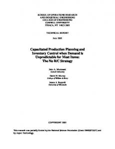
Theorem 3. The optimal control policy is characterized by two ∗ (𝑦), 𝑠𝑝∗ (𝑦)). Specifically, in state state-dependent parameters (𝑠𝑚 (𝑥, 𝑦), (a) it is optimal to manufacture if the serviceable inventory ∗ ∗ ∗ (𝑦). Furthermore, 𝑠𝑚 (𝑦 + 1) ≤ 𝑠𝑚 (𝑦) ≤ level 𝑥 ≤ 𝑠𝑚 ∗ 𝑠𝑚 (𝑦 + 1) + 1; (b) the optimal price control policy is the threshold policy, specially set high price if the serviceable inventory level 𝑥 ≤ 𝑠𝑝∗ (𝑦); otherwise set low price. Furthermore, 𝑠𝑝∗ (𝑦+ 1) ≤ 𝑠𝑝∗ (𝑦). Proof. The manufacturing base-stock level is defined as ∗ (𝑦) = max𝑥 {𝑥 : 𝑉(𝑥 + 1, 𝑦) − 𝑉(𝑥, 𝑦) ≥ 𝑐𝑚 }. Consider 𝑠𝑚 ∗ ∗ ∗ (𝑦) + 1, 𝑦) − 𝑉(𝑠𝑚 (𝑦), 𝑦) ≤ 𝑉(𝑠𝑚 (𝑦) + 1, 𝑦 − 1) − 𝑐𝑚 ≤ 𝑉(𝑠𝑚 ∗ ∗ (𝑦) and P2; 𝑉(𝑠𝑚 (𝑦), 𝑦−1), which is due to the definition of 𝑠𝑚 ∗ ∗ then we have 𝑠𝑚 (𝑦) ≤ 𝑠𝑚 (𝑦 − 1). Furthermore, consider 𝑐𝑚 ≥ ∗ ∗ ∗ ∗ (𝑦) + 1, 𝑦) − 𝑉(𝑠𝑚 (𝑦), 𝑦) ≤ 𝑉(𝑠𝑚 (𝑦), 𝑦 + 1) − 𝑉(𝑠𝑚 (𝑦) − 𝑉(𝑠𝑚 ∗ ∗ 1, 𝑦 + 1) due to P3; then we have 𝑠𝑚 (𝑦 + 1) ≥ 𝑠𝑚 (𝑦) − 1. The price threshold level is 𝑠𝑝∗ (𝑦) = max𝑥 {𝑥 : 𝑉(𝑥+1, 𝑦)− 𝑉(𝑥, 𝑦) ≥ 𝜉}. Consider 𝜉 ≤ 𝑉(𝑠𝑝∗ (𝑦) + 1, 𝑦) − 𝑉(𝑠𝑝∗ (𝑦), 𝑦) ≤ 𝑉(𝑠𝑝∗ (𝑦) + 1, 𝑦 − 1) − 𝑉(𝑠𝑝∗ (𝑦), 𝑦 − 1), which is due to the definition of 𝑠𝑝∗ (𝑦) and P2; then we have 𝑠𝑝∗ (𝑦) ≤ 𝑠𝑝∗ (𝑦−1). Theorem 3 shows that the optimal control policy is statedependent. If it is optimal to manufacture in state (𝑥, 𝑦 + 1), then it is still optimal to manufacture in state (𝑥, 𝑦), but one unit decrease in the core inventory leads to at most one unit increase in the manufacturing base-stock level. This implies that manufacturing control policy depends on the core inventory level. The core inventory and the serviceable inventory are substitutable. The reason is that due to the stochastic of the manufacturing and return processes the core inventory may be restored to the original level during the manufacturing process. It is optimal to set high price when the serviceable inventory level is lower than the threshold level. The threshold level is decreasing at the core inventory level, meaning that if it is optimal to set a high price in state (𝑥, 𝑦), it is still optimal to adopt a high price when the core inventory level is lower than 𝑦. We further visualize the structure of the optimal policy in Figures 2 and 3 using a numerical example. The parameters are 𝛽 = 0.0001, 𝜆 1 = 6, 𝜆 2 = 10, 𝑝1 = 50, 𝑝2 = 40, 𝜇𝑚 = 15, 𝜇𝑟 = 20, 𝑟 = 15, 𝑐𝑚 = 10, 𝑐𝑟 = 5, ℎ𝑟 = 1, ℎ𝑠 = 2, and 𝑏 = 30. The optimal manufacturing policy is shown in Figure 2, while the optimal pricing policy is shown in Figure 3. We specify the optimal action in each region.
4. Conclusions We consider a continuous-review inventory system, in which the serviceable product can be either manufactured or
Mathematical Problems in Engineering
7 The optimality equation can be formulated as
Manufacturing decision
𝑉 (𝑥, 𝑦) = 𝑇𝑉 (𝑥, 𝑦) Do not manufacture X(t)
= −𝐺 (𝑥, 𝑦) + 𝑟𝑉 (𝑥, 𝑦 + 1) + 𝜇𝑟 T𝑟 𝑉 (𝑥, 𝑦)
(31)
+ 𝜇𝑚 T𝑚 𝑉 (𝑥, 𝑦) + T𝑝 𝑉 (𝑥, 𝑦) , Manufacture
where T𝑝 𝑉(𝑥, 𝑦) = max1≤𝑘≤𝑛 {𝜆 𝑘 [𝑝𝑘 + 𝑉(𝑥 − 1, 𝑦)] + ∑𝑖=𝑘̸ 𝜆 𝑖 𝑉(𝑥, 𝑦)}. We can again show that 𝑉(𝑥, 𝑦) preserves properties P1– P3 and characterizes the optimal control policy. For brevity, we ignore the details here. The optimal manufacturing policy possesses a similar structure as the two price cases, while the optimal pricing control policy is given in the following theorem.
Y(t)
Figure 2: The optimal manufacturing policy.
Pricing decision
Theorem 4. The optimal pricing control is characterized by 𝑛 ∗ (𝑦) = regions as follows: there exist 𝑛 price threshold levels; 𝑠𝑝𝑘 max𝑥 {𝑥 : 𝑉(𝑥 + 1, 𝑦) − 𝑉(𝑥, 𝑦) ≥ 𝜉𝑘,𝑘+1 }, 𝑘 = 1, 2, . . . , 𝑛 − 1.
X(t)
Low price
High price
Y(t)
Figure 3: The optimal pricing policy.
remanufactured from the returned product. The system keeps both serviceable and returned product inventory. The lead times of manufacturing and remanufacturing are exponentially distributed. We show that the value function preserves properties P1–P3 and characterizes the optimal pricing and manufacturing policies. Different from the previous literature, we consider pricing decision. The optimal control policy of our model depends on the core inventory level. Specifically, the optimal pricing control policy is the threshold-type policy with threshold level nonincreasing in the core inventory level. The optimal manufacturing control policy is the basestock policy with base-stock level nonincreasing in the core inventory. One possible extension is to consider multiple prices. In this case, the selling price of the serviceable product is chosen among {𝑝𝑘 , 𝑘 = 1, . . . , 𝑛} with 𝑝1 > 𝑝2 > ⋅ ⋅ ⋅ > 𝑝𝑘 > ⋅ ⋅ ⋅ > 𝑝𝑛 . The associated demand arrival rates are {𝜆 𝑘 , 𝑘 = 1, . . . , 𝑛} with 𝜆 1 < 𝜆 2 < ⋅ ⋅ ⋅ < 𝜆 𝑘 < ⋅ ⋅ ⋅ < 𝜆 𝑛 . To facilitate analysis, we further assume that 𝜆 𝑝 − 𝜆 1 𝑝1 𝜆 𝑝 − 𝜆 2 𝑝2 < 𝜉23 = 3 3 < ⋅⋅⋅ 𝜉12 = 2 2 𝜆2 − 𝜆1 𝜆3 − 𝜆2 < 𝜉𝑛−1,𝑛
𝜆 𝑝 − 𝜆 𝑛−1 𝑝𝑛−1 = 𝑛 𝑛 . 𝜆 𝑛 − 𝜆 𝑛−1
There are other research directions worth exploring. First, we can study models with correlated demand and product return processes. This will increase the state space and make the analysis more challenging. Second, the product return is not controllable in our model. We can incorporate and examine the return product acquisition effort decision. Finally, the present model assumes that the remanufactured and manufactured products are the same to customers. But, in some cases, the remanufactured and manufactured products are treated as two different products and sold at different prices. The firm can expand the market share by selling the remanufactured products at a lower price in the low-end market, even though the remanufactured products perform exactly the same function as the new products. In this case, we need to model customer demand by considering how customers choose between these two products. And pricing decisions can be incorporated.
Conflict of Interests The authors declare that there is no conflict of interests regarding the publication of this paper.
Acknowledgment This work was supported in part by the National Natural Science Foundation of China under Grant nos. 71201128, 71201127, and 71302187.
References [1] G. Ferrer and D. C. Whybark, “Successful remanufacturing systems and skills,” Business Horizons, vol. 43, no. 6, pp. 55–64, 2000.
(30)
[2] V. D. R. Guide Jr., “Production planning and control for remanufacturing: industry practice and research needs,” Journal of Operations Management, vol. 18, no. 4, pp. 467–483, 2000.
8 [3] L. Larson, E. O. Teisbeg, and R. R. Johnson, “Sustainable business: opportunity and value creation,” Interfaces, vol. 30, no. 3, pp. 1–12, 2000. [4] D. M. McConocha and T. W. Speh, “Remarketing: commercialization of remanufacturing technology,” Journal of Business & Industrial Marketing, vol. 6, no. 1-2, pp. 23–37, 1991. [5] V. P. Simpson, “Optimum solution structure for a repairable inventory problem,” Operations Research, vol. 26, no. 2, pp. 270– 281, 1978. [6] K. Inderfurth, “Simple optimal replenishment and disposal policies for a product recovery system with leadtimes,” Operations-Research-Spektrum, vol. 19, no. 2, pp. 111–122, 1997. [7] S. X. Zhou, Z. T. Tao, and X. C. Chao, “Optimal control of inventory systems with multiple types of remanufacturable products,” Manufacturing & Service Operations Management, vol. 13, no. 1, pp. 20–34, 2011. [8] Z. Tao, S. X. Zhou, and C. S. Tang, “Managing a remanufacturing system with random yield: properties, observations, and heuristics,” Production and Operations Management, vol. 21, no. 5, pp. 797–813, 2012. [9] G. A. DeCroix and P. H. Zipkin, “Inventory management for an assembly system with product or component returns,” Management Science, vol. 51, no. 8, pp. 1250–1265, 2005. [10] G. A. DeCroix, “Optimal policy for a multiechelon inventory system with remanufacturing,” Operations Research, vol. 54, no. 3, pp. 532–543, 2006. [11] D. P. Heyman, “Optimal disposal policies for a single-item inventory system with returns,” Naval Research Logistics Quarterly, vol. 24, no. 3, pp. 385–405, 1977. [12] J. A. Muckstadt and M. H. Isacc, “An analysis of single item inventory systems with returns,” Naval Research Logistics Quarterly, vol. 28, no. 2, pp. 237–254, 1981. [13] E. Van der Laan and M. Salomon, “Production planning and inventory control with remanufacturing and disposal,” European Journal of Operational Research, vol. 102, no. 2, pp. 264– 278, 1997. [14] E. Van der Laan, M. Salomon, R. Dekker, and L. Van Wassenhove, “Inventory control in hybrid systems with remanufacturing,” Management Science, vol. 45, no. 5, pp. 733–747, 1999. [15] G. A. DeCroix, J.-S. Song, and P. H. Zipkin, “Managing an assemble-to-order system with returns,” Manufacturing & Service Operations Management, vol. 11, no. 1, pp. 144–159, 2009. [16] E. Kim, S. Saghafian, and M. P. Van Oyen, “Joint control of production, remanufacturing, and disposal activities in a hybrid manufacturing-remanufacturing system,” European Journal of Operational Research, vol. 231, no. 2, pp. 337–348, 2013. [17] S. A. Lippman, “Applying a new device in the optimization of exponential queueing systems,” Operations Research, vol. 23, no. 4, pp. 687–710, 1975.
Mathematical Problems in Engineering
Advances in
Operations Research Hindawi Publishing Corporation http://www.hindawi.com
Volume 2014
Advances in
Decision Sciences Hindawi Publishing Corporation http://www.hindawi.com
Volume 2014
Journal of
Applied Mathematics
Algebra
Hindawi Publishing Corporation http://www.hindawi.com
Hindawi Publishing Corporation http://www.hindawi.com
Volume 2014
Journal of
Probability and Statistics Volume 2014
The Scientific World Journal Hindawi Publishing Corporation http://www.hindawi.com
Hindawi Publishing Corporation http://www.hindawi.com
Volume 2014
International Journal of
Differential Equations Hindawi Publishing Corporation http://www.hindawi.com
Volume 2014
Volume 2014
Submit your manuscripts at http://www.hindawi.com International Journal of
Advances in
Combinatorics Hindawi Publishing Corporation http://www.hindawi.com
Mathematical Physics Hindawi Publishing Corporation http://www.hindawi.com
Volume 2014
Journal of
Complex Analysis Hindawi Publishing Corporation http://www.hindawi.com
Volume 2014
International Journal of Mathematics and Mathematical Sciences
Mathematical Problems in Engineering
Journal of
Mathematics Hindawi Publishing Corporation http://www.hindawi.com
Volume 2014
Hindawi Publishing Corporation http://www.hindawi.com
Volume 2014
Volume 2014
Hindawi Publishing Corporation http://www.hindawi.com
Volume 2014
Discrete Mathematics
Journal of
Volume 2014
Hindawi Publishing Corporation http://www.hindawi.com
Discrete Dynamics in Nature and Society
Journal of
Function Spaces Hindawi Publishing Corporation http://www.hindawi.com
Abstract and Applied Analysis
Volume 2014
Hindawi Publishing Corporation http://www.hindawi.com
Volume 2014
Hindawi Publishing Corporation http://www.hindawi.com
Volume 2014
International Journal of
Journal of
Stochastic Analysis
Optimization
Hindawi Publishing Corporation http://www.hindawi.com
Hindawi Publishing Corporation http://www.hindawi.com
Volume 2014
Volume 2014