problem is called double-constrained (see Cung and Hifi, 2000; Lodi and Monaci, ...... Cung, M. Hifi, and B. Le Cun, âConstrained two-dimensional cutting stock ...
Journal of Combinatorial Optimization, 8, 65–84, 2004 c 2004 Kluwer Academic Publishers. Manufactured in The Netherlands. �
Dynamic Programming and Hill-Climbing Techniques for Constrained Two-Dimensional Cutting Stock Problems MHAND HIFI∗ LaRIA, Laboratoire de Recherche en Informatique d’Amiens, Universit´e de Picardie Jules Verne, 5 rue du Moulin Neuf, 8000 Amiens, France Received August 7, 2001; Revised June 6, 2002; Accepted June 7, 2002
Abstract. In this paper we propose an algorithm for the constrained two-dimensional cutting stock problem (TDC) in which a single stock sheet has to be cut into a set of small pieces, while maximizing the value of the pieces cut. The TDC problem is NP-hard in the strong sense and finds many practical applications in the cutting and packing area. The proposed algorithm is a hybrid approach in which a depth-first search using hill-climbing strategies and dynamic programming techniques are combined. The algorithm starts with an initial (feasible) lower bound computed by solving a series of single bounded knapsack problems. In order to enhance the first-level lower bound, we introduce an incremental procedure which is used within a top-down branch-and-bound procedure. We also propose some hill-climbing strategies in order to produce a good trade-off between the computational time and the solution quality. Extensive computational testing on problem instances from the literature shows the effectiveness of the proposed approach. The obtained results are compared to the results published by AlvarezVald´es et al. (2002). Keywords: cutting stock, depth-first search, dynamic programming, hill-climbing, heuristics, knapsacking
1.
Introduction
The efficient and optimal solutions of some medium and large combinatorial optimization problems is highly important for many applications in the field of science and engineering. Using today’s exact methods, sometimes it is not possible to solve some of these instances with amount of computational time. One solution that seems to be attractive is to design robust hybrid approximate algorithms to solve efficiently some large-scale problems, i.e., producing good solutions within reasonable computing time. Cutting and Packing problems belong to an old and very well-known family, called CP in Dyckhoff (1990). This is a family of natural combinatorial optimization problems, admitted in numerous real-world applications from computer science, industrial engineering, logistics, manufacturing, production processes, etc. Long and intensive research on the problems of this family has led (and leads always) to the development of models and mathematical tools, so interesting by themselves that their application domains surpass the framework of CP problems. ∗ Corresponding address: CERMSEM, umr 8095, CNRS, Maison des Sciences Economiques, Universit´ e Paris 1, 106-112 Bd de l’Hˆopital 75647 Paris Cedex 13, France.
66
HIFI
The (un)constrained two-dimensional cutting stock problem (shortly TDC) consists of cutting a given set of small rectangular pieces from a large stock rectangle of fixed dimensions with maximum profit. This problem can also be considered as a subproblem of the general cutting problem in which a set of orders for different pieces has to be met, cutting them from a given set of stock sheets of different sizes. An instance of the TDC problem can be represented by a large stock rectangle R of length L and width W, and a set of type pieces S = {(l1 , w1 ), . . . , (ln , wn )}. Each type i, i = 1, . . . , n, of pieces has a profit ci . In our study we assume that: (i) The pieces have fixed orientation, that is, pieces of dimensions (�, ω) and (ω, �) are not the same. (ii) All cutting tools are of guillotine type, i.e., the vertical and the horizontal cuts (called x-cuts and y-cuts respectively) produce two sub-rectangles. (iii) All the parameters L , W, li and wi , for i = 1, . . . , n, take discrete values. We say that the n-dimensional vector (x1 , . . . , xn ) of integer and nonnegative numbers corresponds to a cutting pattern, if it is possible to produce xi pieces of type i, i = 1, . . . , n, in the large stock rectangle R without overlapping. The TDC consists of determining the cutting pattern with the maximum value, i.e., n � max ci xi TDC = (1) i=1 subject to (x , . . . , x ) corresponds to a cutting pattern 1 n In TDC problem one has, in general, to satisfy a certain demand of pieces. The problem is called unconstrained if these demand values are not imposed, and constrained if the demand is represented by a vector b = (b1 , . . . , bn ), where bi is the maximum number of times that piece of type i, i = 1, . . . , n, can appear in a cutting pattern. In this case, the cutting pattern of equation (1) can be represented by (x1 , . . . , xn ) ≤ (b1 , . . . , bn ). Also, the problem is called double-constrained (see Cung and Hifi, 2000; Lodi and Monaci, 2000) if the demand is represented by two vectors a = (a1 , . . . , an ) and b = (b1 , . . . , bn ), where ai and bi , i = 1, . . . , n, are the minimum and maximum number of times that piece of type i can appear in a feasible cutting pattern. In this case, the cutting pattern of Eq. (1) can be represented by ai ≤ xi ≤ bi , i = 1, . . . , n. Another variant of the TDC problem is to consider a constraint on the total number of cuts, i.e., the sum of some parallel vertical and/or horizontal cuts (using guillotine cuts) does not exceed a certain nonnegative integer k < ∞. In this case the problem is called the staged TDC problem or k-staged TDC problem (see Gilmore and Gomory (1965) and Hifi and Roucairol (2001)). We distinguish two versions of the TDC problem: the unweighted version in which the weight ci of the i-th piece is exactly its area, i.e., ci = li wi , and the weighted version in which the weight of each piece can be independent to its area, i.e., ∃ k ∈ {1, . . . , n} such that ck �= lk wk . Following the classification and notations proposed in Alvarez-Vald´es et al. (2002) and Fayard et al. (1998) for the TDC problem, we study both unweighted and
DYNAMIC PROGRAMMING AND HILL-CLIMBING TECHNIQUES
67
weighted constrained TDC versions: • The Constrained Unweighted version (called CU TDC in Alvarez-Vald´es et al. (2002) and Fayard et al. (1998)): an instance of the problem is defined by the quadruple (R, S, c, b). The value ci of each type i of pieces is equal to its surface ci = li wi . The objective function maximizes the total occupied area, which is equivalent to minimizing the waste (unused area). • The Constrained Weighted version (called CW TDC in Alvarez-Vald´es et al. (2002) and Fayard et al. (1998)): an instance of the problem is defined by the quadruple (R, S, c, b) for which the value ci can be independent from the pieces’s area. In this paper we propose a hybrid approach to deal with the CU TDC and CW TDC problems. This algorithm can be considered as a straightforward extension of the twodimensional unconstrained guillotine cutting approach proposed in Hifi (1997a), with several modifications. The paper is organized as follows. First (Section 2), we present a brief reference of some sequential exact and approximate algorithms for both unconstrained and constrained TDC problems. In Section 3, we describe the main steps of the hybrid algorithm. In Section 3.2, we describe the procedure which is able to produce an initial lower bound used at the top-level of the developed tree. The proposed hybrid algorithm is based upon a top-down approach using a depth-first search strategy (Section 3.1) combined with hill-climbing and dynamic programming techniques (Sections 3.4, 3.5 and 3.6). The hill-climbing strategies are applied in order to produce a good trade-off between the computational time and the solution quality. Finally, in Section 4 the performance of the algorithm is tested on a set of large problem instances and the results are compared with the best known so far. 2.
Sequential algorithms for the TDC problem
Cutting problems have been studied first by Kantorovich (1960) and later used by Gilmore and Gomory (1965, 1966), for commercial and industrial uses. For the cutting stock problem, a large variety of approximate and exact approaches have been devised (see Dyckhoff (1990) and Sweeney and Paternoster (1992)). The constrained TDC problem has been solved exactly by the use of tree-search procedures. Christofides and Whitlock (1977) have proposed a depth-first search method for solving some small problem instances. In Christofides and Hadjiconstantinou (1995) and Hifi and Zissimopoulos (1997) the authors have separately proposed modified versions of Christofides and Whitlock’s approach. In Viswanathan and Bagchi (1993), a generalized exact version of Wang’s approach (1983) has been proposed for both unweighted and weighted cases. The algorithm is principally based upon a best-first search method. In Hifi (1997b), a modified version of Viswanathan and Bagchi’s algorithm has been proposed and in Cung et al. (2000a, 2000b) a better version of the last algorithm has been developed in order to solve some medium and complex problem instances. The unconstrained version of the problem has been solved exactly by applying dynamic programming procedures (see Beasley, 1985; Gilmore and Gomory, 1966; Oliveira and Ferreira,
68
HIFI
1994) and by the use of tree-search procedures (see Herz, 1972; Hifi and Zissimopoulos, 1996). Previous works have also proposed several heuristic approaches to both unconstrained and constrained versions of the problem. For the unconstrained version, Morabito et al. (1992) have proposed a depth-first search and hill-climbing strategies for solving largescale problem instances. Fayard et al. (1998) have designed an algorithm based on solving a series of single knapsack problems using dynamic programming procedures. In Hifi (1997a) a hybrid algorithm, called DHKD algorithm, has been proposed in which the approach of Morabito et al. (1992) and some phases of the method developed in Fayard et al. (1998) were combined. The DHKD algorithm realized good results for large-scale unconstrained TDC problem instances. More recently, Alvarez-Vald´es et al. (2002) have designed some general purpose algorithms for the unconstrained TDC problems. The authors have confirmed the effectiveness of the DHKD algorithm, especially for the large-scale problem instances. For the constrained TDC problem, Wang (1983) proposed a heuristic algorithm which can give an optimal solution under some hypothesis. This algorithm was improved independently by Vasko (1989) and, Oliveira and Ferreira (1990). Arenales and Morabito (1997) and Morabito and Arenales (1996) have extended their previous approach (Morabito et al., 1992) to the constrained case and obtaining good results. Fayard et al. (1998) showed how their approach can also be used for approximately solving the constrained case. The more recent approaches were proposed by Alvarez-Vald´es et al. (2002) in which the authors proposed some large-problem instances and showed that their approaches outperform some existing heuristic algorithms. 3.
The hybrid algorithm for the constrained TDC problem
Branch-and-Bound (B&B) is a well-known technique for solving combinatorial search problems. Its basic scheme is to reduce the problem search space by dynamically pruning unsearched areas which cannot yield better results than already found. The B&B method searches a finite space T, implicitly given as a set, in order to find one state t ∗ ∈ T which is (sub)optimal for a given objective function f. Generally, this approach proceeds by developing a tree in which each node represents a part of the state space T. The root node represents the entire state space T. Nodes are branched into new nodes which means that a given part T � of the state space is further split into a number of subsets, the union of which is equal to T � . Hence, the (sub)optimal solution over T � is equal to the (sub)optimal solution over one of the subsets and the value of the (sub)optimal solution over T � is the minimum (or maximum) of the optima over the subsets. The decomposition process is repeated until the best solution over the part of the state space is reached. 3.1.
The top-down B&B approach
The algorithm is principally based upon a top-down B&B approach using a depth-first search strategy characterizing both CU TDC and CW TDC problems. The main idea of the method is to generate all possible guillotine cutting patterns by developing a tree, where (a) branchings represent cuts on the large rectangle or sub-rectangle, and (b) nodes represent
DYNAMIC PROGRAMMING AND HILL-CLIMBING TECHNIQUES
69
the state of the large rectangle or the current sub-rectangle, after cutting has taken place. For bounding purposes we introduce the following points: (i) (ii) (iii) (iv)
An initial lower bound used at the top-level of the developed tree (see Section 3.2); Intermediary lower bounds used at the inner nodes (see Section 3.4); An upper bound on the maximum value obtainable from each node (see Section 3.5); Hill-climbing strategies which permit to produce a good trade-off between the computational time and the solution quality (see Section 3.6); (v) The optimality-stopping strategy in order to reduce the space search (see Section 3.7).
Several authors (see e.g., Christofides and Whitlock, 1977; Herz, 1972; Hifi, 1997a; Morabito et al., 1992) have used a similar representation and called it the graph (or tree) structure. This type of approach was proposed for solving exactly and approximately some variants of unconstrained and constrained TDC problems. Generally, the search process is considered as a search in a directed graph (or tree), where each (internal) node represents a subproblem and each arc represents a relationship between some nodes. The problem is defined as a search in a graph (or tree) by specifying: (a) the initial node, (b) the final nodes and, (c) the rules that define the allowed moves. As mentioned above, the large rectangle can be represented by the initial node and the pieces by the final nodes. However, each internal node represents a sub-rectangle which represents a part of the initial node. The allowed moves can be considered as the possible cuts on each (sub)rectangle and the different cuts can be applied to the large rectangle which correspond to the degree of this node (R in figure 1, at the top-level). After the cut has taken place, two intermediary nodes are generated which corresponds to two succeeding sub-rectangles. Other cuts can be applied to the resulting internal nodes and so on, until the given sub-rectangles coincide with some pieces. Figure 1 shows the search process used on the directed graph: the nodes B and C (corresponding to two sub-rectangles) are generated by applying a horizontal cut on R, or D and E obtained by using a vertical cut on R; also, the nodes F and G (resp. G and H) are generated by applying a x-cut (resp. y-cut) on C (resp. D). Top−level (root node)
R Large stock rectangle
a horizontal cut
a vertical cut
B
C D
a vertical cut
F
Figure 1.
a horizontal cut
G
The search process used on the directed graph.
H
E
Inner nodes
70 3.2.
HIFI
A lower bound at the top-level
A lower bound on the large stock rectangle can be obtained by applying a modified version of the first phase of the algorithm developed in Fayard et al. (1998) and Hifi (1999). In our study, the problem is reduced into a series of single bounded knapsack problems and solved by using dynamic programming procedures. First, it consists in producing a set of horizontal and vertical strips. Second, two single knapsack problems are solved in order to create a feasible solution. The procedure can be decomposed into two phases. The first phase is composed of two stages: the first stage (Section 3.2.1) is applied in order to construct a set of different horizontal strips and, the second one (Section 3.2.2) is used for combining some horizontal strips in order to produce an approximate horizontal cutting pattern. The second phase of the procedure is also composed of two stages (Section 3.2.3): first, we try to construct a set of vertical strips and we combine some of them for obtaining an approximate vertical cutting pattern. 3.2.1. Construction of the horizontal strips. The problem of generating some horizontal bounded strips can be summarized as follows: without loss of generality, assume that the pieces are ordered in nondecreasing order of widths such that w1 ≤ w2 ≤ · · · ≤ wn . Suppose that (α, β) denotes the current (sub)rectangle, r represents the number of different widths of the considered pieces (i.e., we have the following order w¯ 1 < w¯ 2 < · · · < w¯ r , where ∀ j ∈ {1, . . . , r }, w¯ j ∈ {w1 , . . . , wn }), and (α, w¯ j ) is a strip with width w¯ j ≤ β. We hor define the single Bounded Knapsack problems (B K α, w¯ j ), for j = 1, . . . , r, as follows: � ci xi f whor ¯ j (α) = max i∈Sα,w¯ j � � � hor B K α, w¯ j subject to li x i ≤ α i∈S α, w ¯ j xi ≤ bi , xi is a nonnegative integer, i ∈ Sα,w¯ j where xi denotes the number of times the piece i appears in the j-th horizontal strip without exceeding the value bi , f whor ¯ j (α) is the solution value of the j-th strip, j = 1, . . . , r, and Sα,w¯ j is the set of pieces entering in the strip (α, w¯ j ) such that ∀k ∈ Sα,w¯ j , (lk , wk ) ≤ (α, w¯ j ). Remark 1. It consists in solving a series of small single bounded knapsack problems hor hor hor B K α, w¯ 1 , B K α,w¯ 2 , . . . , B K α,w¯ r , respectively. We can remark that these problems are dependent and their resolution is equivalent to solve only a largest single bounded knapsack hor B K α, w¯ r . This can be realized by using a dynamic programming procedure (Martello and Toth, 1990) and so, we generate r optimal strips with respect to the length of the (sub-)rectangles (α, w¯ i ), where w¯ i ≤ β. 3.2.2. An approximate horizontal cutting pattern. The aim of this step is to select the best of these horizontal bounded strips for obtaining an approximate cutting pattern to both
DYNAMIC PROGRAMMING AND HILL-CLIMBING TECHNIQUES
71
CU TDC and CW TDC problems. We do it by solving another single Bounded Knapsack Problem, given as follows: r � hor (β) = max f whor g ¯ j (α)y j α j=1 � � r � BKPhor (α,β) subject to w¯ j y j ≤ β j=1 y j ≤ a j , y j is a nonnegative integer where y j , j = 1, . . . , r, is the number of occurrences of the j-th horizontal strip in the (sub)rectangle (α, β), bounded by its upper bound-value a j (calculated by using the steps hor described below), f whor ¯ j (α) is the solution value of the j-th strip and gα (β) is the solution value of the cutting pattern, for the (sub)rectangle (α, β), composed of some horizontal strips. We can remark that each horizontal bounded strip j, j = 1, . . . , r, can be appeared at least one time and at most w¯βj times in the large stock rectangle. Let δi j be the number of times that piece of type i appears in the j-th strip. We can easily remark that a possible way for computing each a j , j = 1, . . . , r, is the following: 1. Let F be the set of the different widths w¯ j , j = 1, . . . , r ; Set bi� = bi , i = 1, . . . , n, and K = ∅, where K denotes the set of the widths of the best selected strips. 2. Let w¯ k be the highest width of F, such that there exists i ∈ {1, . . . , n} with δik > 0. If � ∃k then stop, else set K = K ∪ {wk } and set � ak = min
� �
�� bi β , min such that δik > 0 w¯ k 1≤i≤n δik
(2)
3. Reduce the demand values bi� and δi j , i = 1, . . . , n, of each remaining strip j = 1, . . . , |F|, and set F = F \ {wk ∪ {wt : δit = 0, ∀i}}. Of course, the remaining values depend on the value of the current ak given by equation (2). 4. Repeat steps (2) and (3) until F = ∅. Set ak = 0, ∀wk ∈ F \ K . Finally, if one sets α = L and β = W, we obtain the first feasible solution, called approximate horizontal cutting pattern, which is composed of some horizontal bounded (sub)strips. The used (sub) strips are enhanced using the process as illustrated in figure 2. 3.2.3. An approximate vertical cutting pattern. By applying the same process as in Sections 3.2.1 and 3.2.2, we can generate the set of the vertical strips such that: • We consider that pieces are ordered in nondecreasing order such that l1 ≤ l2 ≤ · · · ≤ ln ;
72
HIFI
(a)
(b)
(c)
Figure 2. Illustration of the different solutions obtained by applying three versions of the constructive procedure (the complementary feasible solution).
• We reverse the role of widths and lengths in the previous single bounded knapsack ver hor problems B K α, ¯ j by l¯ j , li by wi , α by β, f whor w¯ j , i.e., w ¯ j (α) by f l¯ j (β) and r by s, where ¯ ¯ s denotes the number of distinct lengths such that l1 < l2 < · · · < l¯s . We denote the resulting single bounded knapsack problems by B K l¯ver , for j = 1, . . . , s. j ,β Also, the second feasible solution, called approximate vertical cutting pattern, is realized by solving the single bounded knapsack problem (BKPver (α,β) ) obtained by reversing the role of widths and lengths in the single bounded knapsack problem (BKPhor (α,β) ). Remark 2. The initial solution value for both CU TDC and CW TDC problems is the one that realizes the best solution value between the approximate horizontal and vertical cutting ver patterns, i.e., the pattern realizing the solution value max{g Lhor (W ), gW (L)}. 3.3.
The discretization procedure
In order to deal with a finite number of cuts, the cuts are made at points which form linear combinations of lengths and widths of pieces, respectively. Herz (1972) showed for the unconstrained TDC problem that the guillotine cuts can, without loss of generality, be integer nonnegative linear combinations of sizes of the ordered pieces. For a given (sub)rectangle (α, β), the cuts can be reduced along the length α (resp. width β) to the following sets: L(α,β) = x | x =
n �
li z i ≤ α, wi ≤ β, z i is a nonnegative integer
i=1
and W(α,β) =
y|y=
n �
wi z i ≤ β, li ≤ α, z i is a nonnegative integer .
i=1
The sets L and W are called discretization (or normalized) sets and each of them can be computed by using the procedure due to Christofides and Whitlock (1977). Hence, in the directed graph, for each generated (sub)rectangle, we consider the cuts corresponding to the points of above sets. In what follows, when we deal with a fixed (sub)rectangle, say (X, Y ), we just consider its normalized rectangle (X 0 , Y0 ), where X 0 = maxx∈L(X,Y ) {x} and Y0 = max y∈W(X,Y ) {y}.
DYNAMIC PROGRAMMING AND HILL-CLIMBING TECHNIQUES
3.4.
73
The lower bound at the inner nodes
Let (α, β) denote the current sub-rectangle and x (resp. y) be a x-cut (resp. y-cut) realized on the length α (resp. width β). This cut generates two sub-rectangles (x, β) and (α − x, β) (resp. (α, y) and (α, β − y)). 3.4.1. A lower bound for the sub-rectangle (x, β) (resp. (α, y)). When we apply the dynamic programming for solving the problem (B K l¯ver ) (resp. (B K Lhor ,w¯ r )), then we create s ,W the longest vertical (resp. highest horizontal) strip. However, all optimal sub-strips (x, β), where x ∈ {l¯1 , . . . , l¯s } and β ≤ W (resp. (α, y), where α ≤ L and y ∈ {w¯ 1 , . . . , w¯ r }), are available, since the single bounded knapsack problem is optimally solved. So, as concerns the intermediary nodes, when we deal with a sub-rectangle, say (x, β) (resp. (α, y)), its lower bound should be obtained by solving two small single bounded knapsack problems. Clearly, if we use such a resolution at each node, then the computational time of the algorithm becomes important, especially for some large-scale problem instances. Then, we propose a simple way which permits us to construct a lower bound for (x, β) (resp. (α, y)) within small computational time. Indeed, when a x-cut (resp. y-cut) is made, we solve both (BKPver x,β ) hor ver hor and (BKPx,β ) (resp. (BKPα,y ) and (BKPα,y )) by using an adaptation of the simple and fast greedy algorithm proposed by Martello and Toth (1990). 3.4.2. A complementary lower bound for (α− x, β) (resp. (α, β − y)). Suppose now that b� realizes the demand vector which represents the structure of the feasible solution on the normalized subrectangle of (x, β) (resp. (α, y)). This solution is obtained by applying the greedy procedure of Section 3.4.1 to the normalized subrectangle of (x, β) (resp. (α, y)). We propose to construct the complementary solution by applying a greedy constructive procedure, as explained herein. The aim of the procedure is to combine a set of horizontal (resp. vertical) (sub-)strips with the remaining pieces, which means that the remaining pieces are placed on the successive horizontal (resp. vertical) strips. Let b�� , where bi�� = bi − bi� , for i = 1, . . . , n, be the vector representing the remaining pieces, such that bi�� > 0 and (li , wi ) ≤ (α − x, β) (resp. (li , wi ) ≤ (α, β − y)). We assume that the pieces are sorted according to decreasing widths (resp. lengths). Of course, if we have two type of pieces, namely k and p, where k �= p, with the same width (resp. length), then we take in first the piece realizing max{ck /(lk wk ), c p /(l p w p )}. In what follows, we describe the procedure only when a y-cut is made. We consider that the first horizontal line is the bottom of the current sub-rectangle. The remaining pieces are placed from left to right with their bottoms at the selected horizontal line. In the other hand, we always apply the vertical placement realizing min{bk�� , ww¯k }, where wk denotes the width of the selected piece, w¯ is the width of the current strip and bk�� represents the remaining demand value of the k-th piece. When a new strip is needed, the corresponding horizontal line is created which coincides with the top of the highest piece placed in the previous strip. The process is iterated until no piece can be placed on a supplementary horizontal strip. The obtained final solution can be considered as the feasible solution of the sub-rectangle (α, β − y), respecting the guillotine cuts. Of course we can also extend the procedure for filling some unused regions of each created strip as for the
74
HIFI
algorithm developed in Fayard et al. (1998) and Hifi (1997a,1999). Limited computational results showed that the above procedure contributes to produce good results, especially for the large-scale problem instances. Figure 2(a) shows a resulting strip when a simple placement is used, figure 2(b) illustrates the resulting strip when the above procedure is applied and, figure 2(c) shows an eventual solution which can be obtained if the extended procedure is applied. 3.5.
The upper bound at the (inner) nodes
In Cung et al. (2000a) and Hifi (1999), we have used an upper bound which can be considered as a generalization of the upper bound used on the surface’s area. Here, we use the same upper bound in the tree-search by calculating another single bounded knapsack. The problem is a linear one and it can be represented as follows: � cjz j U(α, β) = max j∈Rαβ � � u � Subject to (l j w j )z j ≤ (αβ) K α,β j∈Rαβ � � β α z j ≤ min b j , , z j ≥ 0, lj wj
j ∈ Rαβ
where Rαβ is the set of pieces entering in (α, β), z j is the number of occurrences of the j-th piece, where j ∈ Rαβ . u We can remark that (K αβ ), in particular for α = L and β = W, is a large single bounded knapsack. Then, we reorder initially (at the beginning of the algorithm) the elements of the set S in decreasing order such that πc11 ≥ πc22 ≥ · · · ≥ πcnn , where c j and π j are respectively the profit and the surface of the j-th piece and, we apply the greedy procedure for solving u (K α,β ) (we take the upper bound for the sub-rectangle (α, β) the value U(α, β) ). Notice that if we have two terms, say ck /πk and c p /π p , which realize the same coefficient, then we take in first the term with a greater profit, i.e., the index realizing argmax{ck , c p }. 3.6.
Hill-climbing strategies
Let us see now how we can use the previously algorithm for solving efficiently the large CU TDC and CW TDC problem instances. Generally, when the cardinality of the sets of linear combinations L and W is large, then the algorithm becomes computationally infeasible since for each node (α, β) ≤ (L , W ) of the developed tree, it considers O(|α| × |β|) points. In what follows, we describe different strategies which represent the HC (HillClimbing) strategies, applied to the nodes of the developed tree. • We have already mentioned that normalized cutting patterns have been used for reducing the number of combinations on lengths (resp. widths) of the generated (sub)rectangles (nodes). Herz (1972), and Christofides and Whitlock (1977) showed how these sets can be
DYNAMIC PROGRAMMING AND HILL-CLIMBING TECHNIQUES
75
generated by combining the lengths (resp. widths) of the pieces of S. For the unconstrained TDC problem, in Beasley (1985) and Morabito and Arenales (1996), the authors have used a heuristic based upon the previous one for generating a small number of points. In Hifi (1997a) another procedure using the same principle has been proposed. In order to reduce the number of points of both sets L and W, we use the procedure described in Hifi (1997a), with a slight modification. We do it by applying the following function: 0 if i = 0 and x = 0 ∞ if i = 0 and x �= 0 (x) if i �= 0 and ((x
δi�li )) f i (x) = f i−1 � � �� min f i−1 (x), max wi , min x f i−1 (x − kli ) 1≤k≤min{ l ,δi� } i otherwise where 1 ≤ δi� ≤ min{bi , lLi }, for i = 1, . . . , n. For the sub-rectangle (α, β), we affirm that α represents a combination of some lengths of the set S if f n (α) ≤ β (we use the same function for constructing the set of the horizontal points such that we replace δi� by δiw , li by wi and wi by li , where 1 ≤ δiw ≤ min{bi , wWi }, for i = 1, . . . , n). In the hybrid algorithm, we can now limit the number of created nodes by considering the two reduced sets L and W. • Suppose now that a new path is selected by applying a cut on the node A, giving two nodes B and C. For the unconstrained TDC problem, Herz (1972) has suggested a strategy in the tree search procedure that discards some nodes (representing some subrectangles obtained by applying some horizontal or vertical cuts) if a given percentage U(B) + U(C) is less than or equal to L(A), where U(X ) denotes the upper bound of the (sub)rectangle X and L(X ) its lower bound. In Hifi (1997a) and Morabito at al. (1992), this strategy has been extended to the lower bounds. Indeed, if we suppose that the node B terminates by the best lower bound, namely L(B) (in this case, all cuts are examined on this node), then the node C is discarded such that L(B) + �U(C) ≤ L(A), where 0 < � ≤ 1 is a previously given percentage. As for the algorithm developed in Hifi (1997), we apply this strategy by initially setting � to 0.999. • Another HC strategy is to introduce a depth parameter in the tree search procedure. This strategy is a simple and a popular strategy that is based upon local search. It generally elects the best local path and abandons the other suspended paths forever. The proposed algorithm is equipped with a parameter depth which represents the maximum level permitted on the developed tree (see Hifi, 1997a; Morabito et al., 1992). Limited computational experience showed that our algorithm when it uses the depth parameter with values 2 or 3 produced good results within reasonable computational times. 3.7.
Reducing the search space
In this section, we introduce a strategy which permits us to reduce the search space, without affecting the quality of the obtained solution. This strategy permits to neglect the resolution of some single bounded knapsack problems at some internal nodes.
76
HIFI
Proposition. Let (x, β) (resp. (α, y)) be a strip where the first cut is made vertically (resp. horizontally). If x = �min (resp. y = wmin ) or x < 2�min (resp. y < 2wmin ), where �min (resp. wmin ) denotes the smallest length (resp. width) entering in the considered strip, then its optimal solution value is available. Proof: Let x be a vertical cut producing the sub-rectangle (or the strip) (x, β). By solving initially the problem B K (ver , we have necessarily all values f tver (W ), t ∈ {l¯1 , . . . , l¯s }, l¯s ,W ) ver which means that the value f t (β) with β ≤ W, is initially available. Now, if (x, β) is a strip, necessarily there exists an optimal horizontal (sub)pattern containing some pieces (�, w) | �min ≤ � ≤ x and w ≤ β ≤ W. So, we can distinguish the two following cases: 1. If �min = x, then gβver (�min ) = f �ver (β) represents the optimal solution value of (x, β) min since the solution forms the best (uniform) combination of the vertical sub-strips. 2. We prove that if x < 2�min , then gxhor (β) = gβver (x). We can distinguish two cases: (a) Consider that gxhor (β) ≤ gβver (x), which implies that it is not necessary to solve both ver ver problems BKPhor (x,β) and BKP(x,β) for the strip (x, β), since gβ (x) concides with the solution value f �ver (β), where � = max1≤ j≤s {l¯ j | l¯ j ≤ x}. (b) consider that gxhor (β) > gβver (x) = f �ver (x). It means that there exists a partition (x, z) and (x, β − z) such that z ∈ Wx,β for which gxhor (z) + gxhor (β − z) > gβver (x)
(3)
where gxhor (z) denotes the solution value when the problem BKPhor (x,z) is solved. Since ver x < 2�min , then necessary gxhor (z) = gzver (x) = f �ver (z) and gxhor (β − z) = gβ−z (x) = ver � ¯ ¯ f �� (β − z), where � = max1≤ j≤s {l j | l j ≤ x} with wi ≤ β − z, i = 1, . . . , n. So, from Eq. (3) we have ver gzver (x) + gβ−z (x) > gβver (x)
(4)
Equation (4) contradicts the fundamental principle of the dynamic programming. Hence, the solution value of the strip (x, β) is always represented by the value f �ver (x), such that � = max1≤ j≤s {l¯ j | l¯ j ≤ x}, and the demonstration is similar when the cut is made horizontally at the point y. Figure 3 illustrates an optimal (sub)strip which can be obtained at the inner nodes. By considering that the half of the width y (see figure 3(b)) is less than to wmin (figure 3(a): the width of the smallest width-piece entering the (sub)strip (α, y)), then we can remark ver that the best solution of both problems BKPhor (α,y) and BKP(α,y) does not improve the solution hor value f ω¯ (α), where ω¯ = max1≤ j≤r {w¯ j | w¯ j ≤ y}, produced initially by solving the largest hor problem B K (L ,w¯ r ) . Indeed, in this case the union of every partition (α, y1 ) and (α, y − y1 ), where y1 ∈ Wα,y (or (x1 , y) and (α − x1 , y), where x1 ∈ Lα,y ) can not produce a better solution (see Eq. (4) of Proposition).
77
DYNAMIC PROGRAMMING AND HILL-CLIMBING TECHNIQUES
y
wmin (a) Figure 3.
4.
(b)
α
2wmin< y
Illustration of the optimality-stopping strategy.
Computational experiments
The proposed algorithm was coded in C and tested on a UltraSparc10 (250 Mhz and with 128 Mo of RAM). We shall refer to it by TDH, for the Top-Down approach using Hillclimbing strategies. Our computational study was conducted on 82 problem instances of various sizes and densities. These test problems are taken from Alvarez-Vald´es et al. (2002) which are also publicly available from ftp://panoramix.univ-paris1.fr/pub/ CERMSEM/hifi/OR-Benchmark.html. The density of each instance depends on the number of pieces to cut and the number of linear combinations of the sets L and W, respectively. Generally, it means that the complexity of the instance increases if the dimensions of some pieces are reasonably small compared to the dimensions of the large stock rectangle. 4.1.
The problem details
For the weighted case (CW TDC) we have considered 36 problem instances (see Table 1, column 1). The instances CHW1 and CHW2 are taken from Christofides and Whitlock [4], CW1-CW11 are taken from Fayard et al. (1998), four instances (2, 3, A1 and A2) are taken from Hifi (1997b), two other instances (STS2 and STS4) are taken from Tsch¨oke and Holth¨ofer (1995), seven instances (CHL1� ,CHL2-CHL4, Hchl1, Hchl2 and Hchl9) have been considered in Cung et al. (2000). The rest of instances APT40-APT49 are taken from Alvarez-Vald´es et al. (2002), which are generated as follows: the number of pieces to cut is taken uniformly from the interval [25, 60], the dimensions of the stock rectangle L and W are taken from [100, 1000], li (resp. wi ) is taken from [0.05L , 0.4L] (resp. [0.05W, 0.4W ]) and the demand values bi = min{ρ1 , ρ2 }, where ρ1 = L/li W/wi and ρ2 is a number randomly generated in the interval [1, 10]. Also, the value of the weights ci is setting equal to �ρli wi �, where ρ is randomly taken from the interval [0.25, 0.75]. For the unweighted case (CU TDC) we have treated 46 problem instances (see Table 2, column 1). OF1 and OF2 are taken from Oliveira and Ferreira (1990), W from Wang (1983), the instances CU1-CU11 are considered by Fayard et al. (1998), the instances 2s, 3s, A1s, A2s, STS2s, STS4s, CHL1s-CHL4s, CHL5-CHL7, Hchl3s, Hchl4s� , Hchl5s� and Hchl6s-Hchl8s, are taken from Cung et al. (2000), the instances A3-A5 are taken from Hifi (1997b) and the other problem instances (APT30-APT39) are taken from Alvarez-Vald´es et al. (2002), which are generated as for the weighted case. Of course, in this case, each ci , i = 1, . . . , n, is setting equal to the surface area li wi .
78
HIFI
Table 1. The computational results on the weighted problem instances. The symbol ∗ means that the reported value denotes the upper bound of the treated instance, without proof of optimality. The TDH algorithm Instance
Opt/upper∗
CHW1
2892
2892
CHW2
1860
1860
CW1
6402
CW2 CW3
APT algorithm
LB
TDH1
TDH2
2305
2892
2892
1640
1860
1860
6402
6402
6402
6402
5354
5354
5354
5354
5354
5689
5689
5026
5689
5689
CW4
6175
6170
6153
6170
6175
CW5
11659
11644
10683
11659
11659
CW6
12923
12923
12635
12923
12923
CW7
9898
9898
9484
9898
9898
CW8
4605
4605
4318
4605
4605
CW9
10748
10748
10254
10748
10748
CW10
6515
6515
5884
6515
6515
CW11
6321
6321
5747
6321
6321
2
2892
2892
2447
2892
2892
3
1860
1860
1660
1860
1860
A1
2020
2020
1820
2020
2020
A2
2505
2455
2310
2455
2505
STS2
4620
4620
4620
4620
4620
STS4
9700
9700
9414
9700
9700
CHL1�
8671
8660
8040
8660
8660
CHL2
2326
2326
2086
2326
2326
CHL3
5283
5283
4923
5283
5283
CHL4
8998
8998
8000
8998
8998
Hchl1
11303
11089
10444
11184
11255
Hchl2
9954
9918
9398
9941
9953
Hchl9
5240
5240
5060
5240
5240
Small and medium problem instances
Large-scale problem instances APT40
67654∗
66362
64213
67154
67154
APT41
215699∗
206542
202305
206542
206542
APT42
34098∗
33435
33012
33435
33503
APT43
222570∗
214651
212062
214651
214651
APT44
74887∗
73410
70465
73765
73868
APT45
75888∗
74691
74205
74691
74691
APT46
151813∗
149911
147021
149911
149911
APT47
153747∗
148764
142935
149067
150234
APT48
170914∗
166927
165428
167219
167660
APT49
226346∗
215728
202801
216103
218388
79
DYNAMIC PROGRAMMING AND HILL-CLIMBING TECHNIQUES
Table 2. The computational results on the unweighted problem instances. The symbol ∗ means that the reported value denotes the upper bound of the treated instance. The TDH algorithm Instance
Opt/upper∗
APT algorithm
LB
TDH1
TDH2
2737
Small and medium problem instances OF1
2737
2737
2713
2737
OF2
2690
2690
2522
2690
2690
W
2721
2721
2599
2721
2721
CU1
12330
12330
12312
12330
12330
CU2
26100
26100
26100
26100
26100
CU3
16723
16679
16608
16723
16723
CU4
99495
99366
98704
99495
99495
CU5
173364
173364
171651
173364
173364
CU6
158572
158572
158572
158572
158572
CU7
247150
247150
245570
247150
247150
CU8
433331
432714
430368
433331
433331
CU9
657055
657055
657055
657055
657055
CU10
773772
773485
771102
773772
773772
CU11
924696
922161
916730
924696
924696
2s
2778
2778
2393
2778
2778
3s
2721
2721
2599
2721
2721
A1s
2950
2950
2950
2950
2950
A2s
3535
3535
3451
3535
3535
STS2s
4653
4653
4625
4653
4653
STS4s
9770
9770
9481
9770
9770
CHL1s
13099
13099
13036
13099
13099
CHL2s
3279
3279
3198
3279
3279
CHL3s
7402
7402
7072
7402
7402
CHL4s
13932
13932
12638
13932
13932
CHL5
390
390
363
390
390
CHL6
16869
16869
16374
16869
16869
CHL7
16881
16838
16728
16881
16881
Hchl3s
12215
12208
11698
12209
12214
Hchl4s�
11994
11967
10827
11976
11993
Hchl5s�
45361
45223
44311
45283
45361
Hchl6s
61040
61002
60170
61002
61002
Hchl7s
63112
62802
62518
63004
63029
Hchl8s A3
911
904
752
904
904
5451
5436
5403
5436
5436
A4
6179
6179
5885
6179
6179
A5
12985
12929
12449
12963
12976
(Continued on next page.)
80
HIFI
Table 2.
(Continued.) The TDH algorithm Instance
Opt/upper∗
APT30
140904
140144
APT31
824931∗
APT32
38068
APT33
APT algorithm
LB
TDH1
TDH2
140168
140168
140904
814081
821073
822453
823976
38030
37886
38068
38068
236818∗
234920
235580
236611
236611
APT34
362520∗
360084
356159
361042
361167
APT35
622644∗
620700
613656
620843
621021
APT36
130744
130338
129190
130744
130744
APT37
387276
381966
385811
387053
387118
APT38
261698∗
259380
259070
261270
261395
APT39
268750
267168
266378
268020
268750
Large-scale problem instances
4.2.
Computational results
The computational results are shown in Table 1 for the CW TDC problem and in Table 2 for the CU TDC version. The column under Opt/Upper (see Tables 1 and 2, column 2) represents the optimal solutions and in some cases it contains the upper bounds (without proof of optimality). These cases have been marked with a ∗ sign. In this case, we compare the obtained approximate solutions to the upper bound: the upper bound is the solution value realizing min{U(L , W ), H Z (L , W )}, where U(L , W ) is the solution value of the knapsack u problem K (L ,W ) of Section 3.5 and H Z (L , W ) is the solution value of the unconstrained TDC problem, obtained by applying the exact algorithm developed in Hifi and Zissimopoulos (1996). For the other problem instances, the optimal solution values are obtained by applying the exact algorithm developed by Cung et al. (2000). For each problem instance (see Tables 1 and 2), we give, • The optimal (or upper bound) solution value (column 2 of Tables 1 and 2). • The initial lower bound (column 4 of Tables 1 and 2), denoted by LB, produced by applying the pre-processing procedure of Section 3.2 and figure 2. • The approximate solution value produced by both APT (column 3 of Tables 1 and 2) and TDH (columns 5 and 6 of Tables 1 and 2 algorithms. The APT algorithm represents the best algorithm proposed by Alvarez-Vald´es et al. (2002), which is based upon tabu search (called also TABU500 in Alvarez-Vald´es et al. (2002)). Their algorithm is very efficient since it produces, generally, good results within reasonable computational times. The TDH algorithm is denoted by TDH1 when it runs with the parameter depth = 2, and denoted by TDH2 when it is executed with depth = 3. As for the approach proposed in Hifi (1997a), for all treated instances, we reduce the two sets L and
81
DYNAMIC PROGRAMMING AND HILL-CLIMBING TECHNIQUES Table 3.
Summary of computational results on small/medium and large-scale problem instances. Approximation ratios R-APT
R-LB
R-TDH1
Average CPU R-TDH2
T-TDH1
T-TDH2
0.08 53.92 11.07
0.52 71.05 16.96
65.25
121.57
Small and medium weighted problem instances Min Max Av.
0.9800 1 0.9982
Min
0.9531
0.7970 1 0.9279
0.9800 1 0.9987
0.9958 1 0.9998
Large-scale weighted problem instances 0.8960
0.9547
0.9575
Max
0.9875
0.9778
0.9926
0.9926
296.35
445.67
Av.
0.9724
0.9488
0.9735
0.9762
132.97
263.23
Average
0.9913
0.9337
0.9922
0.9937
44.93
85.37
Min
0.9923
0.9923
0.08
0.11
Small and medium unweighted problem instances 0.8255
0.9923
Max
1
1
1
1
41.56
56.95
Av.
0.9987
0.9617
0.9993
0.9995
7.77
11.68
Min
0.9863
0.9963
67.65
121.50
Large-scale unweighted problem instances 0.9825
0.9948
Max
0.9990
0.9962
1
1
282.25
412.30
Av.
0.9929
0.9910
0.9982
0.9989
150.65
260.38
Average
0.9972
0.9700
0.9989
0.9994
38.83
65.75
Global AV.
0.9942
0.9519
41.88
75.56
All treated problem instances 0.9956
0.9965
W by setting the parameters δ1 = δ1� = · · · = δn� (resp. δ2 = δ1w = · · · = δnw ) to 2, where δi� and δiw , for i = 1, . . . , n, are the parameters used in the function described in Section 3.6. Eventually, the reduction of the number of points of both sets L and W reduces the search space, which may degrade the quality of the produced solution. Notice that we have proposed this way because the quality of the solution is recompensed, on one hand, by the quality of the initial lower bound used at the top-level (see Table 3, column 3— it produces an average percentage deviation equal to 5% from the optimum/upper-bound) and, on the other hand, by the intermediary lower bounds. Of course, we can extend the space search by applying a variation on the domain of δ1 and δ2 . In this case, a better solution can be obtained but sometimes a considerable computing time is needed. Examining Tables 1 and 2, we observe that: 1. Over the 62 small and medium problem instances, the TDH1 algorithm found 50 optimal solutions (which represents a percentage of 80.64% with respect to the optimum). Furthermore, the TDH2 algorithm found 53 optimal solutions, while APT approach realizes 44 of the optimal solutions.
82
HIFI
2. Over the 20 large-scale problem instances, the TDH1 algorithm found five better solutions for the weighted case (see Table 1: the instances APT40, APT44, APT47, APT48 and APT49) than the solutions published by Alvarez-Vald´es et al. (2002). Also, the TDH2 algorithm found five better solutions than those reached by the TDH1 version (see Table 1: the instances APT42, APT44, APT47, APT48 and APT49). For the unweighted version of the problem, the same phenomenon is realized. In this case, the TDH1 algorithm produces ten better solutions (see Table 1 column 5) than those published by Alvarez-Vald´es et al. (2002) and, the TDH2 algorithm improves seven solutions (see Table 2 column 6) of the solutions produced by the TDH1 algorithm. 3. For the large-scale unweighted problem instances, the initial lower bound LB produced four better solutions than those produced by the APT algorithm (see Table 2, column 4: the instances APT30, APT31, APT33 and APT37). The computational results of Tables 1 and 2 are summarized in Table 3. We report the average experimental approximation ratios of each algorithm: R-APT for the APT algorithm, R-LB for the lower bound used at the root node, R-TDH1 for the TDH algorithm with the parameter depth = 2, and R-TDH2 when the TDH algorithm is executed with depth = 3. Each experimental approximation ratio is calculated by applying the usual formula A(I )/O pt(I ), where I is an instance of the constrained TDC problem, A(I ) denotes the approximate solution value obtained by each algorithm and O pt(I ) is the optimal (or the upper bound) solution value. The two first blocs of Table 3 summarize the results given by the different algorithms for the small/medium and large weighted problem instances. The next two blocs represent the results for the unweighted version of the problem. Each bloc is represented by a line Min (resp. Max) which represents the minimum (resp. maximum) approximation ratio (or computational time) produced (or consumed) by each algorithm, and another line (Av.), which represents the average approximation ratio (or computational time) over all considered instances. The last line of Table 3 summarizes the global average experimental approximation ratios and the computational times for both weighted and unweighted versions of the TDC problem. From Table 3 we can observe that: • The lower bound: for all treated instances, excellent lower bounds are obtained (by applying the pre-processing procedure of Section 3.2). Over the 62 small and medium problem instances, the approximation ratios varies in the interval [0.797, 1] (resp. [0.8255, 1]) for the weighted (resp. unweighted) case. The average approximation ratio is equal to 0.9279 for the weighted case and equal to 0.9617 for the unweighted one. Over the 20 large-scale problem instances, it realizes an average approximation ratio equal to 0.9488 for the weighted version and equal to 0.9910 for the unweighted case. Globally, over all treated problem instances, the lower bound realizes a good average approximation ratio equal to 0.9519. Therefore, by including these good quality lower bounds and by exploiting some dynamic programming properties, in general tree search procedures, one also expects good behavior from the resulting TDH algorithm. • The TDH1 version: the first version of the algorithm improves significantly the initial lower bound, especially for the large-scale problem instances. In this case, over the 62 small and medium problem instances, the R-TDH1s varies in the interval [0.98, 1] (resp.
DYNAMIC PROGRAMMING AND HILL-CLIMBING TECHNIQUES
83
[0.9923, 1]) for the weighted (resp. unweighted) case. The average R-TDH1 is equal to 0.9987 for the weighted case and equal to 0.9993 for the unweighted one. Over the 20 large-scale problem instances, it realizes a better average R-TDH1 (equal to 0.9858) compared to the results obtained by the APT algorithm. Indeed, the APT algorithm produces an average R-APT equal to 0.9803. Over all treated problem instances, the TDH1 algorithm gives an average R-TDH1 equal to 0.9956, while the APT approach realizes an average R-APT equal to 0.9942. • The TDH2 version: the performance of the second version of the algorithm is remarkably good, especially for the large-scale problem instances. In this case (for the large problems), the average R-TDH2 is equal to 0.9875 within an average computational time equal to 261.81 seconds. We can remark that the algorithm outperforms the APT and the TDH1 algorithms, but it needs more computational times compared to the time consumed by the first version of the TDH algorithm. Over all treated problem instances, the TDH2 algorithm gives an average R-TDH2 equal to 0.9965, while the TDH1 and APT algorithms realize an average approximation ratio equal to 0.9956 and 0.9942 respectively. Finally, the TDH2 algorithm gives these solutions by consuming, on average, 75.56 seconds. 5.
Conclusion
In this paper, we have considered both unweighted and weighted constrained two-dimensional cutting stock problems. We have proposed a hybrid approach combining single bounded knapsack problems, a constructive procedure and hill-climbing strategies. This algorithm can be considered as a straightforward extension of the two-dimensional unconstrained guillotine cutting approach proposed in Hifi (1997a). Empirical evidence for the algorithm has been reported through a number of experiments. These experiments were conducted on different problem instances taken from the literature and show that the algorithm is able to produce good solutions for the large problem instances. Acknowledgment Many thanks to anonymous referees for their helpful comments and suggestions contributing to improve the presentation of the paper. References R. Alvarez-Vald´es, A. Parajon, and J.M. Tamarit, “A tabu search algorithm for large-scale guillotine (un)constrained’ two-dimensional cutting problems,” Computers and Operations Research, vol. 29, no 7, pp. 925–947, 2002. M. Arenales and R. Morabito, “An overview of and-or-graph approaches to cutting and packing problems,” Decision Making under Conditions of Uncertainly, ISBN 5-86911-161-7, pp. 207–224, 1997. J.E. Beasley, “Algorithms for unconstrained two-dimensional guillotine cutting,” Journal of the Operational Research Society, vol. 36, pp. 297–306, 1985. N. Christofides and E. Hadjiconstantinou, “An exact algorithm for orthogonal 2-D cutting problems using guillotine cuts,” European Journal of Operational Research, vol. 83, pp. 21–38, 1995. N. Christofides and C. Whitlock, “An algorithm for two-dimensional cutting problems,” Operations Research, vol. 2, pp. 31–44, 1977.
84
HIFI
V.-D. Cung and M. Hifi, “Handling lower bound constraints in two-dimensional cutting problems,” International Symposium on Mathematical Programming, Atlanta, August 2000. V-D. Cung, M. Hifi, and B. Le Cun, “Constrained two-dimensional cutting stock problems: A best-first branchand-bound algorithm,” International Transactions in Operational Research, vol. 7, pp. 185–210, 2000a. V-D. Cung, M. Hifi, and B. Le Cun, “Constrained two-dimensional cutting stock problems: The NMVB approach and the duplicate test revisited,” Cahiers de la MSE, 2000-127, S´erie Bleue, Universit´e Paris 1. H. Dyckhoff, “A typology of cutting and packing problems,” European Journal of Operational Research, vol. 44, pp. 145–159, 1990. D. Fayard, M. Hifi, and V. Zissimopoulos, “An efficient approach for large-scale two-dimensional guillotine cutting stock problems,” Journal of the Operational Research Society, vol. 49, pp. 1270–1277, 1998. P.C. Gilmore and R.E. Gomory, “Multistage cutting problems of two and more dimensions,” Operations Research, vol. 13, pp. 94–119, 1965. P.C. Gilmore and R.E. Gomory, “The theory and computation of knapsack functions,” Operations Research, vol. 14, pp. 1045–1074, 1966. J.C. Herz, “A recursive computing procedure for two-dimensional stock cutting,” IBM Journal of Research and Development, vol. 16, pp. 462–469, 1972. M. Hifi, “The DH/KD algorithm: A hybrid approach for unconstrained cutting problems,” European Journal of Operational Research, vol. 97, pp. 41–52, 1997a. M. Hifi, “An improvement of Viswanathan and Bagchi’s exact algorithm for cutting stock problems,” Computers and Operations Research, vol. 24, pp.727–736, 1997b. M. Hifi, Contribution a` la r´esolution de quelques probl`emes difficiles de l’optimisation combinatoire, Habilitation Thesis. PRiSM, Universit´e de Versailles St-Quentin en Yvelines, 1999. M. Hifi and C. Roucairol, “Approximate and exact algorithms for constrained (un)weighted two-dimensional two-staged cutting stock problems,” Journal of Combinatorial Optimization, vol. 5, pp. 464–494, 2001. M. Hifi and V. Zissimopoulos, “A recursive exact algorithm for weighted two-dimensional cutting problems,” European Journal of Operational Research, vol. 91, pp. 553–564, 1996. M. Hifi and V. Zissimopoulos, “Constrained two-dimensional cutting: An improvement of Christofides and Whitlock’s exact algorithm,” Journal of the Operational Research Society, vol. 5, pp. 8–18, 1997. L.V. Kantorovich, “Mathematical methods of organizing and planning production,” Management Science, vol. 6, pp. 363–422, 1960. A. Lodi and M. Monaci, “Integer linear programming models for two-staged cutting stock problems,” Technical Report, DEIS, University of Bologna, Italy, 2000. S. Martello and P. Toth, Knapsack Problems, Algorithms and Computer Implementations, John Wiley & Sons Ltd: Chichester, 1990. R. Morabito, M. Arenales, and V. Arcaro, “An and-or-graph approach for two-dimensional cutting problems,” European Journal of Operational Research, vol. 58, no 2, pp. 263–271, 1992. R. Morabito and M. Arenales, “Staged and constrained two-dimensional guillotine cutting problems: An and/orgraph approach,” European Journal of Operational Research, vol. 94, no 3, pp. 548–560, 1996. J.F. Oliveira and J.S. Ferreira, “An improved version of Wang’s algorithm for two-dimensional cutting problems,” European Journal of Operational Research, vol. 44, pp. 256–266, 1990. J.F. Oliveira and J.S. Ferreira, “A faster variant of the Gilmore and Gomory technique for cutting stock problems,” JORBEL, vol. 34, no 1, pp. 23–38, 1994. P.E. Sweeney and E. Paternoster, “Cutting and packing problems: A categorized application-oriented research bibliography,” Journal of the Operational Research and Society, vol. 43, pp. 691–706, 1992. S. Tsch¨oke and N. Holth¨ofer, “A new parallel approach to the constrained two-dimensional cutting stock problem,” in Proceedings of the Second International Workshop. Parallel Algorithms for Irregular Structured Problems, LNCS 980, pp. 285–300, 1995. F.J. Vasko, “A computational improvement to Wang’s two-dimensional cutting stock algorithm,” Computers and Industrial Engineering, vol. 16, pp. 109–115, 1989. K.V. Viswanathan and A. Bagchi, “Best-first search methods for constrained two-dimensional cutting stock problems,” Operations Research, vol. 41, no. 4, pp. 768–776, 1993. P.Y. Wang, “Two algorithms for constrained two-dimensional cutting stock problems,” Operations Research, vol. 31, no. 3, pp. 573–586, 1983.