2011 International Conference on Communication Systems and Network Technologies
Dynamic Programming Approach for Large Scale Unit Commitment Problem Prateek Kumar Singhal
R. Naresh Sharma
Electrical Engineering Department National Institute of Technology, Hamirpur H.P, India
[email protected]
Professor, Electrical Engineering Department National Institute of Technology, Hamirpur H.P, India
[email protected] The organization of the paper is as follows: Section II introduces the UC formulation. Section III shows the method to solve UC based on DP. In Section IV, Simulation results on a 10-unit power generation system is presented and the results are compared with different heuristic techniques and Section V concludes the paper.
Abstract— In this paper, the large scale Unit Commitment (UC) problem has been solved using Dynamic Programming (DP) and the test results for conventional DP, Sequential DP and Truncation DP are compared with other stochastic techniques. The commitment is such that the total cost is minimal. The total cost includes both the production cost and the costs associated with start-up and shutdown of units. DP is an optimization technique which gives the optimal solution. Keywords-unit commitment; dynamic programming; genetic algorithm; lagrange relaxation, simulated annealing, evolutionary programming, binary particle swarm optimization.
I.
INTRODUCTION
Unit Commitment (UC) is used to schedule the generators such that the total system production cost over the scheduled time horizon is minimized under the spinning reserve and operational constraints of generator units. UC problem is a nonlinear, mixed integer combinatorial optimization problem. The global optimal solution can be obtained by complete enumeration, which is not applicable to large power systems due to its excessive computational time requirements [1]. Hence, the UC problem is quite difficult due to its inherent high-dimensional, non-convex, discrete and non-linear nature. The UC problem can be considered as two linked optimization problems, namely the unit-scheduled problem, which is a combinatorial optimization problem and the economic dispatch (ED) problem, which is a non-linear programming optimization problem [2]. There are many UC methods such as the dynamic programming which is introduced in this paper, lagrangian relaxation [3], priority list method, branch and bound method [4] and mixed integer linear programming (MILP) [5]. All of these methods have their advantages and disadvantages. By using dynamic programming for unit commitment, we can get optimal solutions. But solution of large scale UC problems using conventional DP is time consuming because it involves complete enumeration of units instead it gives the best optimal solution [6]. Total no. of combinations for Conventional DP = 2N-1 where ‘N’ is total number of units. In this paper, we will illustrate the components of UC and introduce the solution of UC problem using Conventional dynamic programming, Sequential combination (SC)-DP and Truncation Combination (TC)-DP for 10 unit system over 24 hours interval. 978-0-7695-4437-3/11 $26.00 © 2011 IEEE DOI 10.1109/CSNT.2011.152
UC PROBLEM FORMULATION
II.
The objective of UC problem is to minimize the production cost over the scheduled time horizon (e.g., 24 h) under the generator operational and spinning reserve constraints. Mathematically, the objective function to be minimized is T
N
F P ,U ,
F P
ST , 1
U,
U,
1
subject to following constraints (a) power balance constraint N
P U,
P
0
2
(b) spinning reserve constraint N
P
P,
R
P,
U,
0
3
(c) generation limit constraints U, P P, U , , i 1,2, … N
4
(d) start-up cost ,
= HST , if T , CST , if T ,
T, T,
T, T,
T, ,
, (5)
where, F P – Fuel cost function of the ith unit with generation output P , at hour t. Usually, it is a quadratic polynomial with coefficients a , b and c as follows: a bP c P 2 F P N – Number of units 714
T – Number of hours P – The generation output of the ith unit at hour t ST – Start-up cost of ith unit 0 U , – The on/off status of the ith unit at hour t, and U , 1 when on. when off, U , P - load demand at hour t (in MW) R - spinning reserve at hour t (in MW) - Maximum real power generation of unit i (in MW) P, P, - Minimum real power generation of unit i (in MW) HST - Hot start-up cost of unit i (in dollars) CST - Cold start-up cost of unit i (in dollars) - Minimum down time of unit i (in hours) T, T , - Continuously off time of unit i (in hours) - Cold start hours of unit i (in hours) T, III.
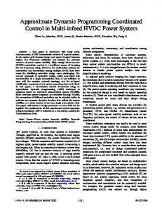
Start
K=1 R K, I
min P
R K, I
min P L
J, K
F
J
1, L
S
K, I
S
K
R K
1, L
1, L: K, I
X= Do for all States I in Period K
Trace Optimal Schedule
1
Stop
Figure 1. UC via forward Dynamic Programming
IV.
J
SIMULATION RESULTS
The results for DP are presented and tested on 10 unit base system with a 24-hour time horizon. The program was written in MATLAB. The input data for 10 unit system and load demands for 24 hours are shown in Tables I and Table II. In this section, a 10-generator, 24-hour unit commitment schedule is determined with the help of Conventional DP, SC-DP and TC-DP and their results consist of production cost and CPU time are compared with different stochastic techniques.
Recursive algorithm to compute the minimum cost in Kth hour with Ith Combination is, L
X= Do for all States I in Period K
Is K=M last hour?
In TC-DP fixed number of units is allowed to run to satisfy the load demand for each hour.
min P
1, L: K, I
Save N lowest cost
Because of this disadvantage, the SC-DP and TC-DP is used to solve the UC problem. The chief advantage of these two methods is the reduction of dimensionality of the problem. Also the calculation of production cost lies near the optimal solution. In SC-DP, the strict priority order of units is imposed. For example, assume the same 4 units, there would be only four combinations to try: Priority 1 Unit Priority 1 Unit + Priority 2 Unit Priority 1 Unit + Priority 2 Unit + Priority 3 Unit Priority 1 Unit + Priority 2 Unit + Priority 3 Unit + Priority 4 Unit
J, K
K
{L} = “N” Feasible States in interval K-1
First, Dynamic programming is a methodical procedure which systematically evaluates a large number of possible decisions in a multi-step problem. When we utilize the existing conventional dynamic programming method, although its solution is correct and has the optimal value, it takes a lot of memory and spends much time in getting an optimal solution [7]-[11]. For example, assume that there are 4 units which can supply the 24 hour load. So, the total maximum path to satisfy the 24 hour load curve is calculated by:
F
S
K=K+1
DYNAMIC PROGRAMMING APPROACH
Total Paths = 2
K, I
L
1, L: J, K
TABLE I.
DATA FOR 10-UNIT SYSTEM [12]
6 Unit 1
Unit 2
Unit 3
Unit 4
Unit 5
Pmax (MW)
455
455
130
130
162
Pmin (MW)
150
150
20
20
25
a ($/h)
1000
970
700
680
450
Parameter
where, J, K – Least total cost to arrive at state (J, K) F J, K – Production cost for state (J, K) P J 1, L: J, K – Transition cost from state (J-1,L) to S State (J, K) State (J, K) – Kth Combination in Jth hour
715
b ($/MWh)
16.19
17.26
16.6
16.5
19.7
c ($/MW2-h)
0.00048
0.00031
0.002
0.00211
0.00398
min up (h)
8
8
5
5
6
min down (h)
8
8
5
5
6
hot start cost ($)
4500
5000
550
560
900 1800
cold start cost ($)
9000
10000
1100
1120
cold start hours (h)
5
5
4
4
4
initial status (h)
8
8
-5
-5
-6
1 0 0 0
Unit6 Unit7 Unit8 Unit9
Unit 6
Unit 7
Unit 8
Unit 9
Unit 10
80
85
55
55
55
20
25
10
10
10
370
480
660
665
670
22.26
27.74
25.92
27.27
27.79
0.0079
0.00413
0.00222
0.00173
3
3
1
1
1
3
3
1
1
1
170
260
30
30
30 60
cold start cost ($)
340
520
60
60
cold start hours(h)
2
2
0
0
0
initial status (h)
-3
-3
-1
-1
-1
TABLE II.
Hour
700
7
1150
13
1400
19
1200
2
750
8
1200
14
1300
20
1400
3
850
9
1300
15
1200
21
1300
4
950
10
1400
16
1050
22
1100
5
1000
11
1450
17
1000
23
900
6
1100
12
1500
18
1100
24
800
3
4
5
6
7
8
9
10
11
12
Unit1 Unit2
1 1
1 1
1 1
1 1
1 1
1 1
1 1
1 1
1 1
1 1
1 1
1 1
Unit3
0
0
0
0
0
0
0
0
1
1
1
1
Unit4
0
0
0
1
1
1
1
1
1
1
1
1
Unit5
0
0
0
0
0
1
1
1
1
1
1
1
Unit6
0
0
0
0
0
0
0
0
0
1
1
1
Unit7
0
0
0
0
0
0
0
0
0
0
0
0
Unit8
0
0
0
0
0
0
0
0
0
0
1
1
Unit9
0
0
0
0
0
0
0
0
0
0
0
1
Unit10
0
0
0
0
0
0
0
0
0
0
0
0
Unit1 Unit2 Unit3 Unit4 Unit5
13 1 1 1 1 1
14 1 1 1 1 1
15 1 1 0 1 1
16 1 1 0 0 1
17 1 1 0 0 1
Hours 18 19 1 1 1 1 0 0 1 1 1 1
20 1 1 1 1 1
21 1 1 1 1 1
22 1 1 1 1 0
23 1 1 0 0 0
0 0 0 0
0 0 0 0
0 0 0 0
0 0 0 0
2
3
4
5
6
7
8
16328 .94
18677 .96
19530 .90
22219 .25
23071 .95
23925 .64
9
10
11
12
13
14
15
16
2630 5.11
28842 .99
30855 .69
32941 .87
28842 .99
26305 .11
23925 .64
20723 .39
17
18
19
20
21
22
23
24
1987 0.09
22219 .25
23925 .64
28842 .99
26305 .11
21910 .82
17182 .48
15476 .40
PRIORITY UNIT LIST
Units
1
2
3
4
5
FLAPC
18.39
19.39
21.98
21.73
22.48
Units
6
7
8
9
10
FLAPC
26.89
33.39
37.92
39.36
39.97
Unit 1 2 3 4 5 6 7 8 9 10
Hours 2
1 0 0 0
14554 .50
TABLE VI.
UNIT COMMITMENT SCHEDULE FOR CONVENTIONAL DP 1
0 0 0 0
PRODUCTION COST FOR EACH HOUR
TABLE V.
A. Results for Conventional DP (Complete enumeration) In this, Table III shows the UC schedule of 10 units over a 24 hours period. Table IV shows the production cost of generators for each hour P ). TABLE III.
0 0 0 0
B. Results for SC-DP In this, the strict priority order of generating units is followed. Table V shows the strict priority order of 10 units based on the full load average production cost. Table VI shows the UC schedule of 10 units over a 24 hours period and Table VII shows the production cost of generators for . each hour (P
Hour
1
0 0 0 0
1
hrs
LOAD DEMAND FOR 24-HOUR [12]
Hour
Hour
0 0 0 0
1368 3.13
hrs
0.00712
hot start cost ($)
0 0 0 0
TABLE IV. hrs
Parameter Pmax (MW) Pmin (MW) a ($/h) b ($/MWh) c ($/MW2-h) min up (h) min down (h)
0 0 0 0
1 1 1 0 0 0 0 0 0 0 0
2 1 1 0 0 0 0 0 0 0 0
3 1 1 0 0 0 0 0 0 0 0
UC SCHEDULE FOR SC-DP
4 1 1 1 0 0 0 0 0 0 0
5 1 1 1 0 0 0 0 0 0 0
6 1 1 1 1 0 0 0 0 0 0
16 1 1 1 1 0 0 0 0 0 0
17 1 1 1 1 0 0 0 0 0 0
18 1 1 1 1 0 0 0 0 0 0
Hours 7 1 1 1 1 0 0 0 0 0 0
8 1 1 1 1 1 0 0 0 0 0
9 1 1 1 1 1 0 0 0 0 0
10 1 1 1 1 1 1 0 0 0 0
11 1 1 1 1 1 1 1 0 0 0
12 1 1 1 1 1 1 1 1 0 0
23 1 1 0 0 0 0 0 0 0 0
24 1 1 0 0 0 0 0 0 0 0
Hours
Unit 1 2 3 4 5 6 7 8 9 10
24 1 1 0 0 0
716
13 1 1 1 1 1 1 0 0 0 0
14 1 1 1 1 1 0 0 0 0 0
15 1 1 1 1 1 0 0 0 0 0
19 1 1 1 1 1 0 0 0 0 0
20 1 1 1 1 1 1 0 0 0 0
21 1 1 1 1 1 0 0 0 0 0
22 1 1 1 1 0 0 0 0 0 0
TABLE VII. Hour
V.
PRODUCTION COST FOR EACH HOUR
1
2
3
4
5
6
7
8
1368 3.13
1455 4.50
1632 8.94
1867 7.96
1953 0.90
2191 0.82
22764. 15
24599. 90
Hour
9
10
11
12
13
14
15
16
2630 5.11
2884 2.99
3114 0.42
3315 3.19
2884 2.99
2630 5.11
24599. 90
21058. 47
Hour
17
18
19
20
21
22
23
24
2020 7.11
2191 0.82
2459 9.90
2884 2.99
2630 5.11
2191 0.82
17182. 48
15476. 40
There are a lot of methods for solving the Unit Commitment problem. Their advantages and disadvantages are studied and described. One of the main problems is that they do not get the optimal solution for performing the Unit Commitment. Therefore, we considered dynamic programming to get an optimal solution despite being impossible to utilize in a large scale power system. This paper presents the three versions of DP to solve UC problem which provide better numerical convergence than other stochastic techniques according to the numerical results. Easy implementation is main attractive feature of all versions of DP.
C. Results for TC-DP In this also the strict priority order is imposed and based on this fixed number of schedulable units are selected to satisfy the load demand for each hour. Number of Units considered = 8 TABLE VIII. Ho urs
Ho urs Ho urs
REFERENCES [1]
PRODUCTION COST FOR EACH HOUR
[2]
1
2
3
4
5
6
7
8
1368 3.13
1455 4.50
16301.8 9
18637 .68
19512 .77
21860 .29
22879 .12
23917 .85
9
10
11
12
13
14
15
16
2618 4.02
2876 8.21
30593.5 1
32550 .09
28768 .21
26184 .02
23917 .85
20895 .88
17
18
19
20
21
22
23
24
2002 0.02
2186 0.29
23917.8 5
28768 .21
26184 .02
21860 .29
17177 .91
15427 .42
[3]
[4]
[5]
[6]
The optimal results are obtained using conventional DP but the computational time taken is more than that of SC-DP and TC-DP. The comparison of production cost and CPU time with other stochastic methods are shown in Table IX. The CPU times may not be directly comparable due to different computers used. CPU times of GA [12] and EP [13] are obtained from HP Apollo 720 workstation and HP C160 workstation, respectively whereas CPU times for LR [12] and SA [14] are obtained from a Pentium IV, 1.6 GHz personal computer and the CPU times for DP are obtained from Intel(R) Core(TM) 2 Duo T6600 @ 2.20 GHz. The CPU time for LR is much smaller compared to other methods. So LR method can provide a fast solution but the quality of solution strongly depends on the algorithm used to update the Lagrangian multipliers. TABLE IX.
[7]
[8]
[9]
[10] [11]
RESULTS FOR DIFFERENT METHODS FOR 10 UNIT SYSTEM OVER 24 HOUR TIME PERIOD
Methods
Overall Production Cost (in $)
CPU Time (in Sec)
Conventional DP SC-DP TC-DP LR [12] GA [12] EP [13] SA [14] BPSO [15]
5,53,507.85 5,55,814.11 5,50,805.02 5,65,825.00 5,65,825.00 5,64,551.00 5,65,828.00 5,63,977.00
458 12 63.3 2.2 221 100 3 18
CONCLUSION
[12]
[13]
[14]
[15]
717
A. J. Wood, and B. F. Wollenberg, Power generation, operation and control, 2nd ed., New York: John Wiley & Sons, 2007, pp. 139. C.K.. Pang, and H.C. Chen, “Optimal short-term thermal unit commitment,” IEEE Transaction on Power Apparatus and Systems, vol. 95, no. 4, pp. 1336-1341, 1976. S. Virmani, K. Imhof, and S. M. Jee, “Implementation of a lagrangian relaxation based unit commitment problem,” IEEE Transaction on Power System, vol. 4, pp. 1373–1379, October 1989. A.I. Cohen, and M. Yoshimura, “A branch-and-bound algorithm for unit commitment,” IEEE Transaction on Power Apparatus and Systems, vol. 102, no. 2, pp. 444-451, 1983. A. C. Williams, “Marginal values in mixed integer linear programming,” Mathematical Programming 44, pp. 67-75, NorthHolland Publishing Company, 1989. G. S. Lauer, N. R. Sandell, D. P. Bertsekas, and T. A. Posbergh, “Solution of large-scale optimal unit commitment problems,” IEEE Transactions on Power Apparatus and Systems, vol. PAS-101, no. 1, pp. 79-86, January 1982. W. L. Snyder Jr., H. D. Powell Jr., and J. C. Rayburn, “Dynamic programming approach to unit commitment,” IEEE Transactions on Power Systems, vol. PWRS-2, no. 2, pp. 339-350, May 1987. C. K. Pang, G. B. Sheble, and F. Albuyeh, “Evaluation of dynamic programming based methods and multiple area representation for thermal unit commitment,” IEEE Transactions on Power Apparatus and Systems, vol. PAS-100, no. 3, pp ,1212-1218, March 1981. Z. Ouyang, and S. M. Shahidehpour, “An intelligent dynamic programming for unit commitment applications,” IEEE Transactions on Power Systems, Paper # 90 SM 468-9 PWRS, 1990. J. A. Momoh, and Yi Zhang, “Unit commitment using adaptive dynamic programming”, ISAP 2005. J. H. Park, S. K. Kim, G. P. Park, Y. T. Yoon, and S.S. Lee, “Modified dynamic programming based unit commitment technique”, IEEE Press, 2010. S. A. Kazarlis, A. G. Bakirtzis, and V. Petridis, “A genetic algorithm solution to the unit commitment problem,” IEEE Transaction on Power System, vol. 11, pp. 83–92, Feburary 1996. K. A. Juste, H. Kita, E. Tanaka, and J. Hasegawa, “An evolutionary programming solution to the unit commitment problem,” IEEE Transaction on Power System, vol. 14, pp. 1452–1459, Nov. 1999. D. N. Simopoulos, S. D. Kavatza, and C. D. Vournas, “Unit commitment by an enhanced simulated annealing algorithm,” IEEE Transaction on Power System, vol. 21, no. 1, pp. 68–76, Feb. 2006. Y.W. Jeong, J.W. Park, S.H. Jang, and K.Y. Lee, “A new quantuminspired binary PSO: application to unit commitment problems for power systems,” IEEE Transaction on Power System, vol. 25, no. 3, pp. 1486–1495, August 2010.