Generalized Leapfrog Scheme for Large-Scale Circuit Simulation Tadatoshi Sekine
Hideki Asai
Graduate School of Science and Technology, Shizuoka University Dept. of Systems Eng., Shizuoka University 3-5-1 Johoku, Naka-ku, Hamamatsu-shi, 432-8561 Japan 3-5-1 Johoku, Naka-ku, Hamamatsu-shi, 432-8561 Japan Phone: +81-53-478-1237, Fax: +81-53-478-1269 Phone: +81-53-478-1237, Fax: +81-53-478-1269 Email:
[email protected] Email:
[email protected] Abstract This paper describes a generalized leapfrog scheme for transient analyses of large-scale circuits. First, the leapfrog scheme developed in the basic latency insertion method (LIM) is described and the characteristics of the method and the scheme are discussed. Then, we propose the generalization technique of the leapfrog scheme which can be applied to the transient analysis of an ill-constructed circuit unsuitable for the basic LIM. Numerical results show that our proposed approach is applicable and efficient for the fast simulation of large-scale networks.
I. I NTRODUCTION Various effects dependent on the high-frequency characteristics of the high-speed signals are induced on the high-density electronic circuits. These effects cause the unexpected behaviors of the chips and packages on a printed circuit board and the errors caused by them seriously affect the signal and power integrity of the network. Thus, it becomes important to verify the electronic circuit behaviors including these effects. In the recent circuit design flow, a net-list for the circuit simulation of such verification is mainly provided by an extractor, which extracts circuit element parameters from the structure and the property of the object to be analyzed. Typically, whenever the extractor is used, the net-list tends to include an enormous number of parasitic elements in order to verify the exact behaviors of the chips and packages. Moreover, it may also include a number of coupling elements such as mutual inductance and branch capacitance because the components in the high-density circuits are very close to each other; they are connected each other electromagnetically, even though they are not connected physically or electrically. These facts cause the large amount of simulation time for a SPICE-like simulator based on the matrix solver. Therefore, fast simulation techniques different from SPICE-like ones are strongly demanded. The latency insertion method (LIM) in [1] has proven to be accurate and extremely fast for the simulation of large networks but suffers from two limitations. The first is that the method requires a circuit to be composed of the branch topology and the node topology both of which must include the reactive elements. The second problem is that since the method is completely explicit, the time step size is restricted by a stability criterion. To overcome these limitations, several enhanced techniques have been proposed [2]–[10]. However, it is still difficult for the basic- and the enhanced-LIM to analyze the ill-constructed circuit such as the circuit without the reactive elements and the tightly coupled elements. The extracted networks may have those undesirable topologies if some kinds of commercial extraction tools such as Q3D Extractor (Ansoft) are used for the extraction. In order to circumvent the limitations of the basic LIM and deal with the ill-constructed circuit, we propose the generalized technique based on the leapfrog scheme for the simulation of large-scale networks. The remainder of the paper is organized as follows. In II, the basic LIM algorithm is reviewed and the characteristics of the method, especially those related to the leapfrog scheme in the algorithm, are discussed. In III, we propose the generalized formulation based on the leapfrog scheme by using the block formulation approach and show the ways how to deal with the ill-constructed topologies to the basic LIM. Section IV shows some numerical results and conclusions are in V. II. L EAPFROG S CHEME IN BASIC LIM In the basic LIM algorithm [1], the circuit to be analyzed is required to be composed of a certain type of the topologies, namely, the branch topology and the node topology as shown in Fig. 1 (a) and (b). Although each branch in the network does not have to contain a resistor Ra,b or a voltage source Ea,b , it must include an inductor La,b . Similarly, each node in the network does not have to contain a conductive path Ga or a current source Ha but must provide a capacitive path Ca to the ground. If there exists a branch without the inductor or a node without the grounded capacitor, a relatively small inductor or shunt capacitor is inserted into the corresponding branch or node to generate the latency, respectively. By this manipulation, the circuit completely consists of the branch topology and the node topology shown in Fig. 1 (a) and (b). Therefore, the all equations derived by applying the Kirchhoff’s voltage law (KVL) to the branch topologies and the Kirchhoff’s current law (KCL) to the node topologies contain derivative terms associated with the reactive elements La,b and Ca as follows: va − vb −
Ma ∑
ia,k
k=1
978-1-4244-4448-9/09/$25.00 ©2009 IEEE 978-1-4244-4448-9/09/$25.00 ©2009 IEEE
dia,b + Ra,b ia,b − Ea,b , dt dva = Ca + Ga va − Ha , dt
= La,b
81 81
(1) (2)
ia , 2 ia ,1 va
La ,b
Ra ,b
E a ,b
vb
Ha
va
vb
node a
ia ,b (b)
branch a,b
Fig. 1. Required circuit topologies for basic LIM. (a) Branch topology. (b) Node topology.
ia ,1
v3
i2 v2
ia ,3
va
vb
ia,b
node a
1 Ra ,b
−1 Ra ,b
0
−1
node b
−1 Ra ,b
1 Ra ,b
0
Ra,b
branch a,b
−1
1
Ra,b
ia,b
−1
1
Fig. 2. Transformation of branch without inductive element. Dark gray parts are not used for stamps.
ia , 2 vint
Cb
1
node b
(a)
vb
ia ,b
Ca
va
Ca Ga
Ra ,b
va
ia , M a
Y2
vint
E2
Fig. 3. Transformation of node without grounded path. First, inductor is transformed into its companion model in time domain. Then, Generalized Y-∆ transformation is applied to remove the intermediate node voltage vint .
i2
Y3
v2
E3
i1 v1
i3
Y1 E1 Fig. 4.
iM a
vM a vint E Y Ma Ma
i1
E2 , 3
Y2,3
i3 v3
Y2, M a
E1, 2 Y1, 2
E1,3
Y3, M a E2 , M a
E3, M a
Y1,3 v1
Y1, M a E1, M a
iM a vM a
Generalized Y-∆ transformation with voltage sources.
where ia,b is the current flowing through the branch between the nodes a and b, va and vb are the voltages at the nodes and Ma is the number of the branches connected to the node a. Then, a finite difference method is applied to (1) and (2) so that the time points of the branch currents and the node voltages are collocated in half time steps, and the updating formulas of the branch current and the node voltage are derived as ) La,b − ∆tRa,b n ∆t ( n+ 12 n+ 12 n+ 12 in+1 = − v + E , (3) i + v a a,b a,b b a,b La,b La,b ) ( M a ∑ Ca ∆t n+ 1 n− 1 (4) va 2 = va 2 + − ina,k + Han , Ca + ∆tGa Ca + ∆tGa k=1
where n is a time step and ∆t is a time step size. All of the branch currents and the node voltages in the network are calculated using (3) and (4) alternately as time progresses. The difference method and the updating process generated in the above basic LIM algorithm is called the “leapfrog scheme” from the viewpoint of the fact that the current and the voltage variables are defined at the different time points where only the current or the voltage exists. By this formulation, if a fixed time step size is used, the calculation amount at each time step results in O(Nb + Nn ), where Nb and Nn are the number of the branches and the nodes in the network, respectively. Therefore, the CPU time of the basic LIM is linearly-increasing with the circuit size, and thereby it can reduce the calculation costs of the transient simulation significantly compared to the SPICE-like algorithm. To clarify the basic LIM algorithm from another perspective, we should realize two principal facts of the method again. One is applying the leapfrog scheme to update the currents and the voltages in the time domain and the other is inserting the artificial latency into the branch and the node with no reactive elements. Additionally, the most important property of the basic LIM is its linear numerical complexity. These facts are the reasons why the latency insertion approach has been introduced in order to generate a scalar version of the leapfrog scheme. In other words, inserting the reactive latency is in fact one of the theoretical techniques to guarantee the linear numerical complexity for updating the variables. Therefore, a primal motivation of the basic LIM seems to be the application of the explicit leapfrog scheme to a transient analysis of large networks. As described above, one of the limitations of the latency insertion approach is the strict restriction of the time step size. The commonly-observed feature on the different stability conditions described in [11] and [7] is that the time step size is restricted by the smallest product of the inductor connected to a node and the grounded capacitor at the node. This condition indicates that if an extremely small reactive latency exists inherently in the network or is inserted artificially, the time step size of the whole system becomes extremely small to guarantee the stability of the method. It is clear that the small time step size induces increasing of the number of the total time steps. If there is the topology which does not have any reactive element, the methods based on the latency insertion approach suffer from the difficulty in achieving a good balance between the acceptable accuracy and the number of the total time steps. As a result, although the latency insertion approach is able to guarantee the linear computational complexity per time step, it may increase the number of the total time steps of the transient analysis significantly due to the extremely small value of, and especially lack of, the latency in networks.
82 82
III. G ENERALIZED L EAPFROG S CHEME The block formulation approach is one of the different techniques from the latency insertion approach. This approach has been developed to deal with the coupled elements such as the branch capacitance in the on-chip power distribution networks (PDNs) [5], [6] and the mutual inductance in the tightly coupled transmission lines [10]. In this section, we expand the approach to deal with more general topologies, especially the circuit without the reactive elements and the tightly coupled elements. The vector-matrix version of the KVL and KCL equations are written as d i + R · i − e, (5) dt d (6) −A · i = C · v + G · v − h, dt where i and v are the vectors of the current and the voltage variables in whole circuit, e and h are the voltage and the current source vector and A is the incidence matrix. These equations are derived by using the RLCG-MNA method [12] in which the associated circuit equation is written as [ ] [ ][ ] [ ] ] [ d v C 0 v h G A · = . (7) + 0 L i e −AT R dt i AT · v
= L·
where the matrices and the vectors are same as those in (5) and (6). It is clear that performing the block matrix operations for (7) is equivalent to calculating two equations (5) and (6). Note that if there is no coupling elements including mutual inductance, branch capacitance and some controlled sources in the circuit and the latency insertion approach is adopted, each matrix in (5) and (6) is a diagonal matrix. Therefore, the explicit leapfrog scheme can be obtained by applying the finite difference method in the basic LIM. However, if the coupling elements exist, the matrices have the dense parts at intervals around the diagonal elements. In the block formulation approach, the variables corresponding to each dense part are solved simultaneously, namely, the implicit leapfrog scheme is generated. In this case, although the dense parts are solved implicitly by using a direct method such as the LU decomposition method, those parts can be separated from each other and also divided from the non-dense parts where the coupling element does not exist. Actually, the implicit leapfrog scheme is more efficient because the matrix solver is applied only to each dense part separately, unlike the conventional direct methods which solve the whole circuit in a lump. Additionally, such an implicit leapfrog scheme can still use the different time step sizes for the different blocks by using the methods in [2] and [8] which are based on the partitioning of the network and the multirate behavior of the network. The coupling elements are induced into the network if the equivalent transformations are performed for the ill-constructed topologies to the basic LIM. For example, the branch without the inductive element is shown in Fig. 2. In the basic LIM, since the resistance Ra,b is a component of the branch topology, its value is stamped into the resistance matrix R associated with the current variable. However, the resistance can be regarded as a conductive pass between the nodes, therefore, its value is stamped into the conductance matrix G associated with the voltage variable. The current variable ia,b is no longer defined at the resistor as shown in Fig. 2. This is in fact equivalent to the partial Gaussian elimination, by which the current variable corresponding to the branch without the reactive elements is eliminated. By this transformation, the stamped part makes a dense block, which is solved by a direct method. Another ill-constructed topology is the node without the capacitive path to the ground shown in Fig. 3. In this case, the transformation by using the companion model of an inductor is applied as shown in Fig. 3, followed by the application of the generalized Y-∆ transformation to remove such an intermediate node. The value of the transformed elements shown in Fig. 4 are defined as Yp Yq Yp,q = ∑Ma , k=1 Yk
Ep,q = Ep − Eq ,
(1 ≤ p < q ≤ Ma ).
(8)
The coupled admittances are induced between the nodes adjacent to the intermediate node in exchange for removing the intermediate node without the grounded capacitance. By these transformations, the ill-constructed topologies are removed and the generalized leapfrog scheme based on the block formulation approach can be applied. The block formulation approach is not restricted by the stability condition in the explicit leapfrog scheme because the extremely small latency is not introduced. IV. N UMERICAL R ESULTS In this section, we apply the generalized leapfrog scheme to an example circuit to estimate the availability of the scheme. The example circuit is shown in Fig. 5. Analysing this type of network is the worst case analysis of the basic LIM because the circuit includes the branch without the inductance and the node without the grounded capacitance. Additionally, the mutual inductances as well as the branch capacitances exist to make tightly coupled connections among the branches and the nodes. The parameters of the grounded and the branch capacitance are Cg = 1.0 pF and Cm = 1.0 fF, respectively, the self inductance is L = 2.0 nH and the mutual inductance is defined as the coupling coefficient K = 0.1. The values of the all resistances are
83 83
Cm
R
L
Cg I in Rin
R
R
L
Cg
R
L
R
L
R R Cg
L
R
R
Cm
K
Cm
Proposed method
K
basic LIM HSPICE
0.1 Voltage [V]
v1
0
L
Cg
−0.1 0
10
20
Time [ns]
Fig. 5. Example circuit. Branch without inductance is in shaded region. Node without grounded capacitance is surrounded by dashed square.
Fig. 6.
Waveform results from v1 .
assigned as R = 0.1 Ω except for the resistance Rin = 50 Ω. We performed the transient analyses using the proposed method, the basic LIM and HSPICE and observed the voltage waveforms of v1 in Fig. 5. In the basic LIM case, the branch capacitance and the mutual inductance are dealt with by the method proposed in [3]. The simulation interval is from 0 ns to 20 ns. The waveform results obtained by each method are shown in Fig. 6. It is confirmed that there is a good agreement between the waveforms from three methods. In this case, the time step size of the proposed method is 1 ps while that of the basic LIM is restricted to 0.477 ps. Thus, the numbers of the total time steps are 20,000 for the proposed method and 41,928 for the basic LIM. As a result, the CPU time of the proposed method is 2.73 seconds and that of the basic LIM is 5.11 seconds, and the CPU costs include the factorization step before the transient analyses. These results indicate that our proposed method is more effective to the ill-constructed circuit. We have already shown the block-LIM is available for the simulation of the large-scale networks including tightly coupled components [10]. It is expected that the proposed method, which is not restricted by the network topologies, is more useful and practical. V. C ONCLUSIONS In this paper, a generalized leapfrog scheme for transient analyses of large-scale circuits has been described. First, the leapfrog scheme developed in the basic latency insertion method (LIM) was described and the characteristics of the method and the scheme were discussed. Then, we proposed the generalization technique of the leapfrog scheme which can be applied to the transient analysis of an ill-constructed circuit to the basic LIM. Some numerical results show that our proposed approach is more suitable for the fast simulation of large-scale networks. ACKNOWLEDGMENT This work is partially supported by NEDO, and the authors would like to thank NEDO for the support in making this work possible. R EFERENCES [1] J. E. Schutt-Ain´e, “Latency insertion method (LIM) for the fast transient simulation of large networks,” IEEE Trans. Circuits Syst. I, vol. 48, pp. 81–89, Jan. 2001. [2] R. Gao and J. E. Schutt-Ain´e, “Improved latency insertion method for simulation of large networks with low latency,” in Proc. IEEE EPEP 2002, Monterey, CA, Oct. 2002, pp. 37–41. [3] Z. Deng and J. E. Schutt-Ain´e, “LIM-SPICE for the analysis of power distribution networks,” in Proc. IEEE SPI 2005, Garmisch-Partenkirchen, Germany, May 2005, pp. 17–20. [4] ——, “Turbo-spice with latency insertion method (LIM),” in Proc. IEEE EPEP 2005, Austin, TX, Oct. 2005, pp. 329–332. [5] J. Choi, M. Swaminathan, N. Do, and R. Master, “Modeling of power supply noise in large chips using the circuit-based finite-difference time-domain method,” IEEE Trans. Electromagn. Compat., vol. 47, pp. 424–439, Aug. 2005. [6] S. N. Lalgudi, Y. Kretchmer, and M. Swaminathan, “Simulation of switching noise in on-chip power distribution networks of FPGAs,” in Proc. IEEE EPEP 2005, Austin, TX, Oct. 2005, pp. 319–322. [7] S. N. Lalgudi, M. Swaminathan, and Y. Kretchmer, “On-chip power-grid simulation using latency insertion method,” IEEE Trans. Circuits Syst. I, vol. 55, pp. 914–931, Apr. 2008. [8] H. Asai and N. Tsuboi, “Multi-rate latency insertion method with RLCG-MNA formulation for fast transient simulation of large-scale interconnect and plane networks,” in Proc. IEEE ECTC 2007, Reno, NV, May 2007, pp. 1667–1672. [9] T. Sekine and H. Asai, “CMOS circuit simulation using latency insertion method,” in Proc. IEEE EPEP 2008, San Jose, CA, Oct. 2008, pp. 55–58. [10] ——, “Block latency insertion method (block-LIM) for fast transient simulation of tightly coupled transmission lines,” in Proc. IEEE EMC Symposium 2009, Austin, TX, Aug. to be published. [11] Z. Deng and J. E. Schutt-Ain´e, “Stability analysis of latency insertion method (LIM),” in Proc. IEEE EPEP 2004, Portland, OR, Oct. 2004, pp. 167–170. [12] Y. Tanji, T. Watanabe, H. Kubota, and H. Asai, “Large scale rlc circuit analysis using RLCG-MNA formulation,” in Proc. DATE’06, Munich, Germany, Mar. 2006, pp. 45–46.
84 84