An optimal dynamic programming algorithm for POSGs .... Once QT i is computed, standard techniques for selecting equilibria in normal form games can be ...
Dynamic Programming Approximations for Partially Observable Stochastic Games Akshat Kumar and Shlomo Zilberstein Department of Computer Science University of Massachusetts Amherst, MA 01002, USA
Abstract Partially observable stochastic games (POSGs) provide a rich mathematical framework for planning under uncertainty by a group of agents. However, this modeling advantage comes with a price, namely a high computational cost. Solving POSGs optimally quickly becomes intractable after a few decision cycles. Our main contribution is to provide bounded approximation techniques, which enable us to scale POSG algorithms by several orders of magnitude. We study both the POSG model and its cooperative counterpart, DEC-POMDP. Experiments on a number of problems confirm the scalability of our approach while still providing useful policies.
Introduction Partially observable stochastic games (POSGs) provide a general, powerful paradigm for decentralized decision making by a group of agents. POSGs allow agents to have conflicting goals in their general form or to share a common reward structure as in DEC-POMDPs (Bernstein et al. 2002). While there has been some progress with applying stochastic games in multi-agent planning and learning (Boutilier 1999), research on stochastic games with partial observability has been sparse. Partial observability is particularly useful when agents cannot completely observe their environment or when different agents perceive different observations. Examples include soccer playing robots, multirobot coordination (Seuken and Zilberstein 2007a) and broadcast channel protocols (Bernstein et al. 2002). An optimal dynamic programming algorithm for POSGs has been developed by Hansen, Bernstein, and Zilberstein (2004). Dynamic programming for POSGs resembles in some ways POMDP solution techniques, but subtle yet significant differences disallow the direct import of POMDP algorithms. Value iteration for a POMDP works by transforming it into a completely observable continuous-state MDP over belief states. However, in POSGs, the environment state changes as a function of the joint action of all agents. Since agents do not have access to other agents policies during plan execution, they cannot maintain the same kind of belief state statistics. This problem is alleviated by introducing the notion of a generalized belief state (Hansen, Bernc 2009, Association for the Advancement of Artificial Copyright Intelligence (www.aaai.org). All rights reserved.
stein, and Zilberstein 2004). That is, agents maintain a belief over the underlying state as well as over the policies of other agents. The optimal algorithm, however, quickly becomes intractable beyond a small horizon (≈4) (Hansen, Bernstein, and Zilberstein 2004). The main aim of our work is to increase the scalability of dynamic programming algorithms by multiple orders of magnitude. We achieve this by providing a memory bounded representation of the value function defined over the generalized belief space. Our technique also provides an error bound over the optimal policies. Such techniques were shown to be successful in the POMDP domain (Feng and Hansen 2001; Varakantham et al. 2007) and we extend them to POSGs. Finite horizon cooperative POSGs or DEC-POMDPs have been shown to be NEXP-complete (Bernstein et al. 2002). DEC-POMDP algorithms (Seuken and Zilberstein 2007b) are similar to dynamic programming for general POSGs. Additionally, they exploit the cooperative nature of the agents to introduce heuristics that prune a large part of the search space. We use our approximation techniques in conjunction with an existing approach, MBDP (Seuken and Zilberstein 2007b). MBDP works within a pre-specified memory bounds, but it requires exponential space in the number of agents and number of observations. Our improvement, MBDP-AS, has the anyspace characteristic and is much more scalable than MBDP. Experiments on a particularly large problem show the effectiveness of MBDP-AS in finding near optimal policies w.r.t. MBDP, using up to an order of magnitude less space.
Background This section introduces the POSG model. For details we refer to (Hansen, Bernstein, and Zilberstein 2004).
Partially observable stochastic games A partially observable stochastic game can be defined as a tuple hAg, S, b0 , {Ai }, {Oi }, P, {Ri }i • • • •
Ag is a finite set of agents indexed 1, . . . , n S is a finite set of environment states b0 ∈ ∆(S) is the initial state distribution Ai is the finite set of actions for agent i. The joint action → − a ∈ ×i∈Ag Ai is given by ha1 , . . . , an i
• Oi is a finite set of observations for agent i. The joint → observation − o ∈ ×i∈Ag Oi is given by ho1 , . . . , on i • P is a set of state transition and observation probabilities. → → → P(s0 , − o |s, − a ) is the probability of taking joint action − a 0 in state s resulting in transition to state s and receiving → joint observation − o → − → − • Ri : S × A → < is the reward function for agent i, A is the set of all joint actions. At each step of the game, the agents simultaneously choose actions, receive a reward and an observation. The environment transitions stochastically into a different state and the above process repeats. The goal for each agent is to maximize the expected sum of rewards it receives during the game. In DEC-POMDPs, the reward function Ri is the same for all agents requiring them to work cooperatively. A policy for an agent is a mapping from local observation histories to actions. Policies can be represented as trees. In a policy tree, the root node defines the action taken at time step t = 0. The edges of the tree represent the possible observations and lead to a new action which will be executed upon receiving that observation. The depth of the tree defines the horizon T of the problem. Generalized belief state Since agents do not communicate during execution time, they do not directly observe other agents policies and cannot maintain the belief over environment states. A generalized belief is defined for each agent i, which maintains a belief over the underlying state as well as the policies of other agents. It is described by a distribution over S × Q−i , where Q−i is the set of policies of all other agents. The distribution is denoted by bi . The generalized belief space for agent i is denoted by Bi . The value of agent i’s belief is given by X Vi (bi ) = max bi (s, q)Vi (s, p, q−i ) p∈Qi
s∈S,q−i ∈Q−i
where Qi is the set of policies of agent i. Assuming two agents, Vi (s, p, q) is the value of agent i’s policy p when other agent executes its policy q and the environment is in state s. It can be easily calculated from problem specifications. Similar to POMDPs, the value function Vi for agent i is |S × Q−i | dimensional, piecewise linear and convex. Dynamic programming for POSGs We describe briefly dynamic programming over generalized belief states. Given depth-t policy trees Qti for each agent i, the multi-agent backup operator H performs the exhaustive backup of these trees to get Qt+1 . Then it recursively computes the geni eralized value function Vit+1 . Subsequently, iterated elimination of dominated strategies is performed for each agent i. This step is unique for POSGs and not applicable to POMDPs. The domination condition is ∀b ∈ Bi , ∃vk ∈ Vit+1 \vj s.t. b.vk ≥ b.vj
(1)
The weakly dominated strategies represented by vj are eliminated from the respective policy tree sets, and this process continues iteratively by alternating over agents until there are no further changes. The above DP algorithm converts
the POSG to a normal form representation with reduced set of strategies. Once QTi is computed, standard techniques for selecting equilibria in normal form games can be applied.
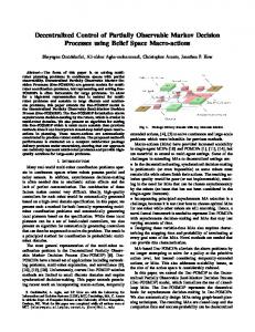
Bounded approximation using � pruning The key issue in the complexity of the DP algorithm is the size of the vector set representing a value function after performing the backup. The size of this vector set is reduced by the iterated elimination of dominated strategies but it still remains a key source of complexity. Our approximation techniques further reduce this vector set size by introducing an error of at most �. The first approximation technique prunes the policies which are higher valued than the remaining policies by at most �. This technique is easy to implement but it is somewhat limited as it does not prune every possible vector allowed by the � error threshold. The next approximation we propose mitigates this shortcoming and reduces the size of the vector set further. We start by defining the notion of � dominated set followed by the first approximation technique EPrune. Definition 1. The vector set Γ representing the value function V is � dominated by the set Γ0 representing V 0 iff V (b) + � ≥ V 0 (b) for the given � and any b. Γ is �parsimonious if removal of any additional vectors from Γ violates the � domination condition i.e., Γ is the minimal such set. We describe below an approximation algorithm EPrune which returns an � dominated set V corresponding to the set U produced by the backup operator H. 1. Choose an agent i 2. Initialize the set Vi with the dominant vectors at belief simplex. 3. Choose a vector u ∈ Ui according to ordering Θ, use the linear program shown in Algorithm 1 to find if u �dominates Vi at any belief point b. If not, discard u. 4. Compute u0 , the best vector at b, remove it from Ui and add it to Vi . Repeat steps 3, 4 until Ui is empty. The above algorithm is run iteratively for each agent i until no more pruning is possible. Each iteration of EPrune introduces an error of at most � over the set U. For detailed proof we refer to (Varakantham et al. 2007). Proposition 1. For a given ordering Θ of the vectors in the set U, EPrune is not guaranteed to return a parsimonious � dominated set V (per iteration). Proof. The proof is by a counterexample. Figure 1(a) shows a simplified vector set U defined over two states s1 and s2 . The individual numbers identify respective vectors. � Algorithm 1: �DOM IN AT E(α, U, �) 1 variables:δ, b(s)∀s ∈ S 2 maximize δ P 3 Ps b(s)[α(s) − u(s)] ≥ δ + � ∀u ∈ U 4 s∈S b(s) = 1 5 if δ ≥ 0 return b else return null
!
!
#
1
1
1
>!
>! 2
"
$!
$"
(a)
3
3
s1
s2
2
s1
(b)
s2
s1
(c)
s2
(d)
s1
s2
(e)
Figure 1: a) shows the vector set U. b) through d) show the steps of algorithm EPrune. e) Shows the � dominated parsimonious set for U. is shown alongside as a line of length �. Consider the ordering Θ = {1, 2, 3} for the vectors in U. During step 1 of EPrune, suppose we choose to initialize the set V with the leftmost belief point. The best vector for this corner, 1, is included in the current representation of V (Figure 1(b)). Step 2 of EPrune selects the next vector, 2, in Θ. Since 2 dominates the current set V by more than � (Figure 1(c)), it will not be pruned by Algorithm 1. The remaining vector, 3, from U, is considered next and it also dominates current V by more than � (Figure 1(d)), so is retained in V . However we can easily see that V is not parsimonious though � dominated (Figure 1(d)). We can remove vectors 1 and 2 from V without affecting the � domination condition. The � dominated parsimonious set is shown in Figure 1(e). An important implication of proposition 1 is that algorithm EPrune is sensitive to the ordering Θ used. For a different ordering Θ0 = {3, 1, 2} for the set U in Figure 1(a), we will get the correct parsimonious �-dominated set shown in 1(e). Out next approximation technique improves EPrune by further reducing the vector set size keeping the error fixed.
IEPrune: improved epsilon pruning The improved epsilon pruning scheme is based on better use of the ordering of vectors in the set U for pruning. IEPrune prunes much more vectors than EPrune while retaining the same error �. For a given upper bound on the size of approximate vector set V, we can pack more useful vectors in V, thereby reducing the error � than in EPrune. Algorithm 3 shows the code for IEPrune. It takes as input the vector set U, the error threshold �, ordering Θ of vectors in U and a user defined parameter k. It returns the � dominated set V for U. IEPrune can be logically divided into three phases. Phase 1 (lines 6-10) is similar to EPrune which removes all vectors which dominate V by less than �. In the next two phases, IEPrune tries to identify if more vectors can be removed keeping the error fixed. During phase 2, it determines potential group of k vectors which can be removed from V without increasing the error � (using Algorithm 2) and stores them in the Cliques set. In phase 3, it removes all the vectors in the Cliques set from V preemptively, adds back any vector which violates the � domination condition. Phase 2:. This part forms the basis for Phase 3; it identifies heuristically the potential candidate vector sets which can be further pruned from V. The accuracy of the heuristic
Algorithm 2: is�Consistent(X, V, �)
3
forall v ∈ X do if �DOM IN AT E(v, V, �) null then Return false
4
Return true
1 2
depends on the parameter k. The set S denotes this potential set (line 11). It contains all subsets of size k of V, with |V| |S| = Ck . In the block lines 13-15, we try to identify which members of S if removed from V will still make the set V � consistent. To ensure this, we also have to take into account the vectors removed in previous iterations (each run of the repeat-until block), stored in the set W (line 13). Set Cliques contains the resulting vectors. Phase 3: A candidate set is constructed which denotes all vectors that potentially can be further pruned (line 16). We preemptively remove all the vectors in candidates set from V (line 17), and later add any vector that fails the is�Consistent test ensuring that the error � doesn’t increases (line 22). The above iteration continues until there are no more vectors in U, and the resulting set V is returned.
Analysis of IEPrune Proposition 2. IEPrune provides a � dominated set V over U i.e. ∀b ∈ B V(b) + � ≥ U(b) where V(.) and U(.) represent the respective value function. Proof. Phase 1 of IEPrune is the same as EPrune, so any vector removed at this phase from the set V is � dominated. For proof see (Varakantham et al. 2007). After this there are two cases possible: In the first case, IEPrune does not prune any additional vectors. Hence the set V remains � dominated. In the second case, IEPrune removes additional vectors to EPrune. Recall that V represents a value function and V(b) = maxv∈ΓV b.v. V is the final representation which is obtained at the end of phase 3 for each iteration. We prove the proposition by contradiction. Suppose that ∃b ∈ B s.t. V(b) + � < U(b). Let vb� = arg maxv∈ΓV b.v and vb? = arg maxv∈ΓU b.v for the current representation of V, U. Also our assumption implies vb� 6= vb? and vb? ∈ / V. We have vb� .b + � < vb∗ .b ⇒ vb∗ .b > vb� .b + � (2)
Optimal Horizon # of Policy Policies Value 2 (6, 6) 2.00 3 (20, 20) 2.99 4 (300, 300) 3.89 5 8 10 100 -
Algorithm 3: IEPrune ( U, �, Θ, k) 1 Returns: the set V � dominated by U 2 3 4 5 6 7 8 9 10 11 12 13 14 15
16 17 18 19 20 21 22
23 24
25
V ← (remove) Best vectors from U at belief simplex W ← φ, Cliques ← φ repeat v ← Θ(U) b ← �-DOMINATE(v, V, �) if b = null then Skip to next iteration v 0 ← (remove) Best vector at b from U V ← V ∪ v0
Candidates ← ∪i si | si ∈ Cliques V 0 ← V\Candidates P runed ← φ forall v ∈ Candidates do X ← {v} ∪ W if ¬is�Consistent(X, V 0 , �) then V 0 ← V 0 ∪ {v} else P runed ← P runed ∪ {v} W ← W ∪ P runed
Consider the case when vb∗ was considered by IEPrune. If it was removed during phase 1, then the � domination proof of phase 1 contradicts our assumption. So surely it must have been removed during phase 3. This implies vb? ∈ Candidates and consequently vb? passed the is�Consistent test (line 21) to be eligible for pruning. From the condition of LP-DOMINATE in is�Consistent test we have: ∃˜ v ∈ V 0 @b ∈ B s.t. vb? .b ≥ δ + � + v˜.b and δ ≥ 0
IEPrune
Random
2.00 2.99 3.89 4.79 7.49 9.29 73.10
2.00 2.99 3.89 4.79 7.49 9.29 82.10
1 1.49 1.99 2.47 3.93 4.90 48.39
Table 1: Comparison of the scalability of different approaches over the MABC problem
S ← {{vi }|vi ∈ V ∧ |{vi }| = k} forall s ∈ S do X ← s ∪ W , V 0 ← V\s if is�Consistent(X, V 0 , �) then Cliques ← Cliques ∪ s
V ← V 0, until U = φ Return V
EPrune
(3)
At any point during the iteration of for loop (20-23) the following holds: V 0 ⊆ V and since vb� is the best vector in V at the belief b, we have vb� .b ≥ v˜.b. Combining this with eq 3 and substituting δ = 0, we get @b ∈ B s.t. vb? .b ≥ � + vb� .b. This is a contradiction to our assumption in Eq. 2. Hence the proposition must hold. It can be shown that the error � accumulates during each invocation of IEPrune like EPrune (Varakantham et al. 2007).
POSG experiments We experiment on Multi access broadcast channel (MABC) domain introduced in (Hansen, Bernstein, and Zilberstein 2004) and compare the performance of EPrune, IEPrune
with the optimal dynamic programming. The MABC problem involves two agent which take control of a shared channel for sending messages and try to avoid collisions. Table 1 shows the comparison of optimal dynamic programming with the approximation schemes. The space requirements for optimal DP become infeasible after horizon 4. In our approximation schemes, we bounded the number of policies to 30 per agent and epsilon value was increased until the policy tree sets were within the required size. Table 1 clearly shows the increased scalability of the approximation techniques. Their performance matched with the optimal policy until horizon 4. Using the bounded memory, these schemes could execute up to horizon 100 (possibly even further), multiple orders of magnitude over the optimal algorithm. When comparing with a random policy, even for larger horizons the approximations provided useful policies achieving nearly 200% of the random value. The next experiment was performed on the larger multiagent tiger problem (Seuken and Zilberstein 2007b). Figure 2 shows the comparison of IEPrune and EPrune on total error and � value used for each horizon. We show the relative percentage of the total error accumulated and the � per horizon i.e. �IEP rune /�EPrune × 100. The graph clearly shows that IEPrune prunes more vectors and packs more useful vectors within the given space requirements thereby reducing the total error and � than EPrune. The next section describes application of IEPrune for DEC-POMDPs resulting in an any space algorithm for solving DEC-POMDPs.
Any-space dynamic programming for DEC-POMDPs DEC-POMDPs are a special class of POSGs which allow cooperative agents to share a common reward structure. The number of possible policies per agent is of the order T O(|A||O| ) for horizon T . This explains why effective pruning is crucial to make algorithms scalable. Recently, a memory bounded dynamic programming approach MBDP has been proposed for DEC-POMDPs (Seuken and Zilberstein 2007b). MBDP limits the number of policy trees retained at the end of each horizon to a predefined threshold M axT rees. The backup operation produces |A|M axT rees|O| policies for each agent for the next iteration. MBDP then uses a portfolio of top-down heuristics to select M axT rees belief points and retains only the best
110
Epsilon value Total Error
100 90 80
% values
70 60 50 40 30 20 10 5
10
15
20
25
30
35
40
45
50
Horizon
Figure 2: IEPrune versus EPrune: % total error and � value used for each horizon Algorithm 4: MBDP-Prune({Qi }, M axJointP olicies) 1 2 3 4 5 6 7 8 9
JointPolicies ← |Q1 ||Q2 | repeat forall agent i ∈ Ag do Sizei ← M axJointP olicies/|Q−i | Q0i ← Randomly select Sizei policies from Qi evaluate(Q0i , Q−i ) IEPrune(VQ0i , �, Θ, k) IncreaseEpsilon? JointPolicies ← |Q1 ||Q2 | until JointPolicies≤ M axJointP olicies
policies for each agent per sampled belief. To further reduce the complexity (Carlin and Zilberstein 2008) use partial backups in their approach MBDP-OC and limit the number of possible observations to a constant M axObs. This results in |A|M axT reesM axObs policies for the next iteration per agent. MBDP provides significant speedups over existing algorithms but has exponential space complexity in the observation space. We use the improved epsilon pruning scheme IEPrune to make MBDP any space: MBDP-AS, and also provide a bound on the error produced by IEPrune over MBDP.
MBDP-AS MBDP-AS takes a user defined parameter M axJointP olicies which restricts MBDP-AS to store only M axJointP olicies joint policies, effectively reducing the space requirements from |A|2 M axT rees2·M axObs to |S|M axJointP olicies for two agents. MBDP-AS introduces an extra step of pruning shown in Algorithm 4 just after the backup operation. Algorithm 4 prunes policies of each agent until the total joint policies is within the limit M axJointP olicies. After this pruning step all agents evaluate their policies against each other requiring only O(|S|M axJointP olicies) space and retain the best policies for the beliefs sampled by the top-down heuristic. We describe the Algorithm 4 in the following. The motivation behind Algorithm 4 is that many policy
vectors which provide similar rewards can be pruned while retaining only a representative subset of them. Such systematic pruning requirement is ideally achieved with IEPrune. We call each execution of pruning (lines 4-9) an iteration of MBDP-Prune. To avoid evaluating every joint policy for agent i, we select a random subset of i’s policies such that current total joint policies are within M axJointP olicies limit (lines 4,5). These joint policies are then evaluated (line 6). For the |S × Q−i | dimensional multi-agent belief b, the policy vector associated with agent i’s policy p is given by V (p) = (. . . , V (p, q−i , s) . . .), q−i ∈ Q−i , s ∈ S. The set of all policy vectors of agent i is passed to IEPrune (line 7) which gives a smaller � dominated set. For all the vectors which are pruned by IEPrune we also prune the corresponding policies from Qi . We then decide if to increase � (line 8) to aggravate the pruning considering the time overhead, and if no policy was pruned in the last iteration. This iterative pruning continues until the JointP olicies are within the specified limit.
Analysis of the MBDP-Prune operation Proposition 3. The maximum number of iterations required by the MBDP-Prune operation is (∆ − �)/δ, where � is the initial epsilon value used, δ is the increment in epsilon after� each iteration. ∆ = maxb∈BM minVi ∈VQi (Vb? .b − Vi .b) and Vb? = argmaxVi ∈VQi Vi .b for any b. Proof. The MBDP-Prune operation will continue to increase epsilon (line 8) by the amount δ until the current joint policies are within M axJointP olicies limit. The worst case is when there is only one policy vector V 0 allowed. V 0 must dominate all other vectors at some multi-agent belief i.e. ∃b s.t. (V 0 .b − Vi .b) ≥ 0 ∀Vi ∈ VQi , V 0 6= Vi . The quantity (V 0 .b − Vi .b) must be the maximum for all belief points so that setting epsilon to that value requires IEPrune to prune every vector other than V 0 . This amount is given by ∆. Consequently, the number of iterations required to raise epsilon to ∆ are (∆ − �)/δ. Proposition 4. Each iteration of MBDP-Prune results in joint policy values that are at most � below the optimal joint policy value in MBDP for any belief state. This results directly from proposition 2. For further details we refer the reader to (Amato, Carlin, and Zilberstein 2007). Proposition 4 forms the basis of quality guarantees over the approximation. If n iterations of MBDP-Prune are required to bring down the joint policies within the limit, the maximum error at any belief is bounded by n� over MBDP with no pruning.
MBDP-AS experiments We built MBDP-AS on top of MBDP-OC (Carlin and Zilberstein 2008) which is similar to MBDP except that it uses partial backups. The test problem we use is cooperative box pushing (Carlin and Zilberstein 2008), which is substantially larger than other DEC-POMDP benchmarks such as Tiger and Multiagent Broadcast Channel (Seuken and Zilberstein 2007b). In this domain, two agents are required to push boxes into the goal area. Agents have 4 available actions and
horizon 5 10 20 30 40 50
Joint Policies=11664 IMBDP MBDP-OC 79 72 91 103 96 149 89 168 68 244 81 278
Joint Policies=2500 MBDP-AS 69 93 148 170 228 268
Table 2: Comparison of IMBDP, MBDP-OC, MBDP-AS on the Repeated Box Pushing domain with various horizons (with MaxTrees = 3, MaxObs = 3) horizon 5 10 20 40
Joint Policies=2500 MaxTree = 3 69 93 148 228
Joint Policies=7000 MaxTree = 4 77 105 150 248
Table 3: Comparison of MBDP-AS for two settings: MaxTree=3 and MaxTree = 4. MaxObs=3 in both cases can receive 5 possible observations. The number of states is 100. Full backups in MBDP are costly, so IMBDP (Seuken and Zilberstein 2007a) and MBDP-OC (Carlin and Zilberstein 2008) take partial backups with M axObs observations. We compare all three algorithms IMBDP, MBDP-OC and MBDP-AS on two metrics: space requirements, which is shown by the total number of joint policies stored and the best policy value. Table 2 compares all three algorithms on these metrics. MBDP-OC and IMBDP evaluate and store all 11664 joint policies, whereas in MBDP-AS we set the M axJointP olicies = 2500, which is nearly one fifth of the total policies. Even at this greatly reduced policies the quality of policies in MBDP-AS is comparable to MBDPOC. We only lose slightly for higher horizons (40-50) on MBDP-OC while always superior to IMBDP for nearly all horizons. This clearly depicts the effectiveness of MBDPAS which prunes selectively using IEPrune algorithm. In the next set of experiments, M axT rees was increased to 4. This requires both IMBDP and MBDP-OC to store and evaluate 65536 policies and is infeasible due to excessive memory requirements. MBDP-AS still scaled well using M axJointP olicies = 7000, about an order of magnitude less policies than total joint policies. Table 3 compares the result for MBDP-AS with M axT rees = 3 and M axT rees = 4. As expected the quality of solution increased for all horizons with the number of MaxTrees. This further confirms the scalability of our approach and effectiveness of MBDP-Prune operation. As far as execution time is concerned MBDP-AS provided interesting results. The average time per horizon for M axT rees = 3 and M axObs = 3 for MBDP-OC was 470sec. For MBDP-AS with the same parameters the average execution time per horizon was 390sec. The overhead of linear programs used for pruning was more than compensated by the lesser policy evaluations which MBDP-AS
performed. Total policy evaluations in MBDP-OC per horizon was 2 × 11664 = 23328. MBDP-AS on the contrary evaluates only M axJointP olicies at one time and prunes many policies. The effort to evaluate pruned policies in the next iteration is saved, leading MBDP-AS to evaluate 16300 policies on average.
Conclusion Our work targets the dynamic programming bottleneck which is a common problem associated with value iteration in DEC-POMDPs and POSGs. We have improved an existing epsilon pruning based approximation technique and our improvement provides better error bound across all horizons on the examined tiger problem. As a second application of our new pruning technique, we incorporate it into an existing algorithm, MBDP, for DEC-POMDPs and address a major weakness of it: exponential space complexity. The new algorithm MBDP-AS is an any-space algorithm, which also provides error bounds on the approximation. Experiments confirm its scalability even on problem sizes where other algorithms failed. These results contribute to the scalability of a range of algorithms that rely on epsilon pruning to approximate the value function.
Acknowledgments This work was supported in part by the AFOSR under Grant No. FA9550-08-1-0181 and by the NSF under Grant No. IIS-0812149.
References Amato, C.; Carlin, A.; and Zilberstein, S. 2007. Bounded dynamic programming for Decentralized POMDPs. In Proc. of AAMAS workshop on Multi-agent sequential decision making in uncertain domains, 31–45. Bernstein, D.; Givan, R.; Immerman, N.; and Zilberstein, S. 2002. The complexity of decentralized control of Markov Decision Processes. Mathematics of Operations Research 27:819–840. Boutilier, C. 1999. Sequential optimality and coordination in multiagent systems. In Proc. of International Joint Conference on Artificial Intelligence, 478–485. Carlin, A., and Zilberstein, S. 2008. Value-based observation compression for DEC-POMDPs. In Proc. of International Conference on Autonomous Agents and Multiagent Systems, 501–508. Feng, Z., and Hansen, E. 2001. Approximate planning for factored POMDPs. In Proc. of European Conference on Planning. Hansen, E. A.; Bernstein, D. S.; and Zilberstein, S. 2004. Dynamic programming for partially observable stochastic games. In Proc. of AAAI, 709–715. Seuken, S., and Zilberstein, S. 2007a. Improved memorybounded dynamic programming for decentralized POMDPs. In Proc. of Conference on Uncertainty in Artificial Intelligence. Seuken, S., and Zilberstein, S. 2007b. Memory-bounded dynamic programming for DEC-POMDPs. In Proc. of International Joint Conference on Artificial Intelligence, 2009–2015. Varakantham, P.; Maheswaran, R.; Gupta, T.; and Tambe, M. 2007. Towards efficient computation of error bounded solutions in POMDPs: Expected Value Approximation and Dynamic Disjunctive Beliefs. In Proc. of International Joint Conference on Artificial Intelligence, 2638-2644.