partially observable Markov ON/OFF channels. In this network instantaneous channel states are never known, and at most one user is selected for service in ...
11
Network Utility Maximization over Partially Observable Markovian Channels
arXiv:1008.3421v1 [math.OC] 20 Aug 2010
Chih-ping Li, Student Member, IEEE and Michael J. Neely, Senior Member, IEEE IEEE
Abstract—We consider a utility maximization problem over partially observable Markov ON/OFF channels. In this network instantaneous channel states are never known, and at most one user is selected for service in every slot according to the partial channel information provided by past observations. Solving the utility maximization problem directly is difficult because it involves solving partially observable Markov decision processes. Instead, we construct an approximate solution by optimizing the network utility only over a good constrained network capacity region rendered by stationary policies. Using a novel frame-based Lyapunov drift argument, we design a policy of admission control and user selection that stabilizes the network with utility that can be made arbitrarily close to the optimal in the constrained region. Equivalently, we are dealing with a high-dimensional restless bandit problem with a general functional objective over Markov ON/OFF restless bandits. Thus the network control algorithm developed in this paper serves as a new approximation methodology to attack such complex restless bandit problems.
provides partial partial information information of of from ACK/NACK feedback provides to improve improve user user selection selection future states, which can be used to performance. Our Our goal goal is is to to design design decisions and network performance. maximizes aa general general network network a network control policy that maximizes the achieved achieved throughput throughput utility metric which is a function of the the amount amount of of user-n user-n data data vector. Specifically, let ynn(t) be the y for user throughput y for user nn served in slot t, and� define the throughput n n Pt−1 )]. Let Λ be the network , limt→∞ 1t1t t−1 E [y (τ )]. Let Λ be the network as y n � n n τ =0 τ =0 uplink, defined defined as as the the closure closure of of capacity region of the wireless uplink, N vectors yy � , (y (ynn))N Then the set of all achievable throughput vectors n=1.. Then n=1 utility maximization maximization problem: problem: we seek to solve the following utility
I. I NTRODUCTION NTRODUCTION This paper studies a multi-user wireless scheduling problem over partially observable environments. We consider a wireless uplink system serving N users via N independent Markov ON/OFF channels (see Fig. 1). Suppose time is slotted with
The problem (1)-(2) is very important important to to explore explore because because itit fields. In In multi-user multi-user wirewirehas many applications in various fields. network utility utility over over stochastic stochastic less scheduling, optimizing network under the the assumption assumption that that networks is first solved in [1], under and are are known known perfectly perfectly and and channel states are i.i.d. over slots and consider here here generalizes generalizes instantly. The problem (1)-(2) we consider framework in in [1] [1] to to networks networks the network utility maximization framework capability (see (see [?], [2], [2] [3] and and referreferwith limiting channel probing capability channel state state information information ences therein) and delayed/uncertain channel [4]–[6] and references therein), therein), in in which which we we shall shall take take (see [3]–[5] [7] to improve improve network network perforperforadvantage of channel memory [6] making, (1)-(2) (1)-(2) also also captures captures mance. In sequential decision making, bandit problems problems [7] [8] in in which which an important class of restless bandit two-state restless restless bandit, bandit, each Markovian channel represents a two-state and packets served over a channel are are rewards rewards from from playing playing the bandit. This class of Markov ON/OFF ON/OFF restless restless bandit bandit problems has modern applications in in opportunistic opportunistic spectrum spectrum access in cognitive radio networks networks [9], [8], [10] [9] and and target target tracking tracking of unmanned aerospace vehicles [10]. [11]. Solving the maximization problem problem (1)-(2) (1)-(2) is is difficult difficult bebecause Λ is unknown. In principle, we we may may compute compute Λ Λ by by locating its boundary points. However, However, they they are are solutions solutions to to N N-dimensional Markov decision processes processes with with information information state state N , where ω (t) is the conditional vectors ω(t) � , (ωnn(t))N ωnn (t) is the conditional n=1 n=1 probability that channel n is ON in slot slot tt given given the the channel channel observation history. Namely, let snn(t) (t) denote denote the the state state of of channel n in slot t. Then
Pn,10 Pn,11
ON(1)
OFF(0)
Pn,00
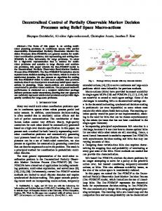
Pn,01 Fig. 1. The Markov ON/OFF chain for channel n ∈ {1, 2, . . . , N }.
normalized slots t ∈ Z+ . Channel states are fixed in every slot, and can only change at slot boundaries. In every slot, the channel states are unknown, and at most one user is selected for transmission. The chosen user can successfully deliver a packet if the channel is ON, and zero otherwise. Since channels are ON/OFF, the state of the used channel is uncovered by an error-free ACK/NACK feedback at the end of the slot (failing to receive an ACK is regarded as a NACK). The states of each Markovian channel are correlated over time, and thus the revealed channel condition Chih-ping Li (web: http://www-scf.usc.edu/∼chihpinl) and Michael J. Neely (web: http://www-rcf.usc.edu/∼mjneely) are with the Department of Electrical Engineering, University of Southern California, Los Angeles, CA 90089, USA. This material is supported in part by one or more of the following: the DARPA IT-MANET program grant W911NF-07-0028, the NSF Career grant CCF-0747525, and continuing through participation in the Network Science Collaborative Technology Alliance sponsored by the U.S. Army Research Laboratory.
g(y) maximize: g(y) ∈Λ Λ subject to: y ∈
(1) (1) (2) (2)
g(·) aa generic generic utility utility function function where in the above we denote by g(·) nonnegative, and and nondecreasing. nondecreasing. that is concave, continuous, nonnegative,
ωn (t) � , Pr [sn (t) = ON | channel observation observation history] history] .. (3) (3)
We will show later ωnn(t) takes values values in in aa countably countably infinite infinite set. Thus computing Λ and solving (1)-(2) (1)-(2) seem seem to to be be infeainfea-
2
sible. Instead of solving (1)-(2), in this paper we adopt an achievable region approach to construct approximate solutions to (1)(2). The key idea is two-fold. First, we explore the problem structure and construct an achievable throughput region Λint ⊂ Λ rendered by good stationary (possibly randomized) policies. Then we solve the constrained maximization problem: maximize: g(y)
(4)
subject to: y ∈ Λint
(5)
as an approximation to (1)-(2). This approximation is practical because every throughput vector in Λint is attainable by simple stationary policies, and achieving feasible points outside Λint may require solving the much more complicated partially observable Markov decision processes (POMDPs) that relate to the original problem. Thus for the sake of simplicity and practicality, we shall regard Λint as our operational network capacity region. Using the rich structure of the Markovian channels, in [12], [13] we have constructed a good achievable region Λint rendered by a special class of randomized round robin policies. It is important to note that we will maximize g(y) only over this class of policies. Since every point in Λint can be achieved by one such policy (which we will show later), equivalently we are solving (4)-(5). We remark that solving (4)-(5) is decoupled from the construction of Λint . We will show in this paper that (4)-(5) can be solved. Therefore, the overall optimality of this achievable region approach depends on the proximity of the inner bound Λint to the full capacity region Λ. The main contribution of this paper is that, using the Lyapunov optimization theory originally developed in [14], [15] and later generalized by [1], [16] for optimal stochastic control over wireless networks (see [17] for an introduction), we can solve (4)-(5) and develop optimal greedy algorithms. Specifically, using a novel Lyapunov drift argument, we construct a frame-based, queue-dependent network control algorithm of service allocation and admission control.1 At the beginning of each frame, the admission controller decides how much new data to admit by solving a simple convex program.2 The service allocation decision selects a randomized round robin policy by maximizing an average MaxWeight metric, and runs the policy for one round in the frame. We will show that this joint policy stabilizes the network and yields the achieved network utility g(y) satisfying g(y) ≥ g(y ∗ ) −
B , Vg
(6)
where g(y ∗ ) is the optimal objective of (4)-(5), B > 0 is a finite constant, Vg is a predefined positive control parameter, and we temporarily assume that all limits exist. By choosing Vg sufficiently large, we can approach the optimal utility g(y ∗ ) arbitrarily well in (6), and thus solve (4)-(5). Restless bandit problems with Markov ON/OFF bandits have been studied in [18]–[20], in which index policies [8], 1 Admission
control is used to facilitate the solution to the problem (4)-(5). admission control decision decouples into N separable onedimensional problems that are easily solved in real time in the case when g(y) is a sum of one-dimensional utility functions for each user. 2 The
[21] are developed to maximize long-term average/discounted rewards. In this paper we extend this class of problems to having a general functional objective that needs to be maximized. This new problem is difficult to solve using existing approaches such as Whittle’s index [8] or Markov decision theory [22], because they are typically limited to deal with problems with very simple objectives. The achievable region approach we develop in this paper solves (approximately) this extended problem, and thus could be viewed as a new approximation methodology to analyze similar complex restless bandit problems. In the next section we introduce the detailed network model. Section III summarizes the construction of the inner bound Λint in [12], [13]. Our dynamic control algorithm is developed in Section IV, and the performance analysis is given in Section V. II. D ETAILED N ETWORK M ODEL In addition to the basic network model given in Section I, we suppose every channel n ∈ {1, . . . , N } evolves according to the transition probability matrix � � Pn,00 Pn,01 Pn = , Pn,10 Pn,11
where state ON is represented by 1 and OFF by 0, and Pn,ij denotes the transition probability from state i to j. We suppose every channel is positively correlated over time, so that an ON state is likely to be followed by another ON state. An equivalent mathematical definition is xn , Pn,01 + Pn,10 < 1 for all n. Let Pn be known by both the network and user n. We suppose every user has a data source of unlimited packets. In every slot, user n ∈ {1, . . . , N } admits rn (t) ∈ [0, 1] packets from the source into a queue Qn (t) of infinite capacity. For simplicity, we assume rn (t) takes real values in [0, 1] for all n.3 Define r(t) , (rn (t))N n=1 . At the beginning of every slot, the network chooses and sends to the users one feasible admitted data vector r(t) according to some admission policy. We let Qn (t) and µn (t) ∈ {0, 1} denote the queue backlog and the service rate of user n in slot t. Assume Qn (0) = 0 for all n. Then the queueing process {Qn (t)} evolves as Qn (t + 1) = max[Qn (t) − µn (t), 0] + rn (t).
(7)
The network keeps track of the backlog vector Q(t) , (Qn (t))N n=1 in every slot. We say queue Qn (t) is (strongly) stable if t−1 1X E [Qn (τ )] < ∞, lim sup t→∞ t τ =0 and the network is stable if all queues in the network are stable. Clearly a sufficient condition for stability is: t−1 N
1 XX lim sup E [Qn (τ )] < ∞. t→∞ t τ =0 n=1
(8)
Our goal is to design a policy that admits the right amount of packets into the network and serves them properly, so that 3 We can accommodate the integer-value assumption of r (t) by introducn ing auxiliary queues; see [1] for an example.
3
the network is stable with utility that can be made arbitrarily close to the optimal solution to (4)-(5). III. A P ERFORMANCE I NNER B OUND In this section we summarize the results in [12], [13] on constructing an achievable region Λint using randomized round robin policies. See [13] for detailed proofs. A. Sufficient statistic As discussed in [23, Chapter 5.4], the information state vector ω(t) defined in (3) is a sufficient statistic of the network, meaning that it suffices to make optimal decisions based only on ω(t) in every slot. (k) For channel n ∈ {1, . . . , N }, we denote by Pn,ij the kstep transition probability from state i to j, and πn,ON its stationary probability of state ON. Since channels are posi(k) tively correlated, we can show that Pn,01 is nondecreasing and (k) (k) Pn,11 is nonincreasing in k, and πn,ON = limk→∞ Pn,01 = (k) limk→∞ Pn,11 . For channel n, conditioning on the outcome of the last observation and when it was taken, it is easy to see that ωn (t) takes values in the countably infinite set (k) (k) Wn , {Pn,01 , Pn,11 : k ∈ N} ∪ {πn,ON }. Let n(t) be the channel observed in slot t via ACK/NACK feedback. The evolution of ωn (t) for each n then follows: Pn,01 , if n = n(t), sn (t) = OFF ωn (t + 1) = Pn,11 , if n = n(t), sn (t) = ON ωn (t)Pn,11 + (1 − ωn (t))Pn,01 , if n 6= n(t). (9) B. Randomized round robin Let Φ denote the set of all N -dimensional binary vectors excluding the zero vector 0. Every vector φ , (φn )N n=1 ∈ Φ stands for a collection of active channels, where we say channel n is active in φ if φn = 1. Let M (φ) denote the number of 1’s (or active channels) in φ. Consider the following dynamic round robin policy RR(φ) that serves active channels in φ possibly with different order in different rounds. This is the building block of the randomized round robin policies that we will introduce shortly. Dynamic Round Robin Policy RR(φ): 1) In each round, suppose an ordering of active channels in φ is given. 2) When switching to active channel n, with probability (M (φ)) Pn,01 /ωn (t) keep transmitting packets over channel n until a NACK is received, and then switch to the (M (φ)) next active channel. With probability 1−Pn,01 /ωn (t), transmit a dummy packet with no information content for one slot (used for channel sensing) and then switch to the next active channel. 3) Update ω(t) according to (9) in every slot. It is shown in [24] that, when channels have the same transition probability matrix, serving all channels by a greedy round robin policy maximizes the sum throughput of the network. Thus we shall get a good achievable throughput
region Λint by randomly mixing round robin policies, each of which serves a different subset of channels. Consider the following randomized round robin that mixes RR(φ) policies for different φ: Randomized Round Robin Policy RandRR: 1) P Pick φ ∈ Φ ∪ {0} with probability αφ , where α0 + φ∈Φ αφ = 1. 2) If φ ∈ Φ is selected, run RR(φ) for one round with the channel ordering of least recently used first. Then go to Step 1. If φ = 0, idle the system for one slot and then go to Step 1. For notational convenience, let RR(0) denote the operation of idling the system for one slot. For any φ ∈ Φ, we note (M (φ)) that the RR(φ) policy is feasible only if Pn,01 ≤ ωn (t) whenever we switch to active channel n. This condition is enforced in every RandRR policy by serving active channels in the order of least recently used first [13, Lemma 6]. Consequently, every RandRR is a feasible policy.4 We note that the RandRR policies considered here are a superset of those in [13], because here we allow the additional idling operation. This enlarged policy space, however, has the same achievable throughput region as that in [13], because idle operations do not improve throughput. We generalize the RandRR policies here to ensure that every feasible point in Λint can be achieved by some RandRR policy. It is also helpful to note that, for any φ ∈ Φ and a fixed channel ordering, every RR(φ) policy is a special case of the randomized round robin RandRR with αφ = 1 and 0 otherwise. C. The achievable region Next we summarize the achievable region rendered by randomized round robin policies. Theorem 1 ([12], [13]). For each vector φ ∈ Φ, define the (φ) N -dimensional vector η (φ) , (ηn )N n=1 where M (φ) (1−(1−xn ) )/(xn Pn,10 ) Pn,01P , if φn = 1 Pn,01 (1−(1−xn )M (φ) ) ηn(φ) , M (φ)+ n:φn =1 xn Pn,10 0, if φn = 0 and xn , Pn,01 + Pn,10 . Then the class of RandRR policies supports all throughput vectors λ in the set n �� �o Λint , λ | 0 ≤ λ ≤ µ, µ ∈ conv η φ φ∈Φ ,
where conv (A) denotes the convex hull of set A, and ≤ is taken entrywise. Corollary 1. When channels have the same transition probability matrix so that Pn = P for all n, we have: !) ( � � cM (φ) φ , Λint = λ | 0 ≤ λ ≤ µ, µ ∈ conv M (φ) φ∈Φ
4 The feasibility of RandRR policies is proved in [13] under the special case that there are no idle operations (α0 = 0). Using the monotonicity of (k) (k) k-step transition probabilities {Pn,01 , Pn,11 }, the feasibility can be similarly proved for the generalized RandRR policies considered here.
4
the network. We will use the Lyapunov optimization 4 theory to construct a dynamic policy that learns a near-optimal P01 (1 − (1 − x)M (φ) ) cM , x = P01 + P10 , solve solution (4)-(5), where the closeness to the true optimality (4)-(5)toby admission control and service allocation in where (φ) � M (φ) x P10 + P01 (1 − (1 − x) ) the network. We will use the Lyapunov optimization theory M (φ) is controlled by a positive control parameter V . g (10) P01 (1 − (1 − x) ) , x = P01 + P10 , c (φ) , M due (φ) ) to channel and M we havexdropped the symmetry. to construct a dynamic policy that learns a near-optimal P10 + P01 (1subscript − (1 − x)n
where
(10) solution to (4)-(5), where the closeness to the true optimality Constructing Lyapunov drift controlled by a positive control parameter Vg . Thewe closeness of thetheinner bound Λint toand the full capacity is A. and have dropped subscript n due channel symmetry.
region Λ is quantified in [12] in the special case that channels We start with constructing a frame-based Lyapunov driftof the inner bound Λmatrix. int and the haveThe the closeness same transition probability Forfull anycapacity feasible A. minus-utility over a frame of size T , where T is Constructing inequality Lyapunov drift region Λ is quantified in [13] in the special case that channels direction v, it can be shown that as v becomes more sym- possibly random but has a finite second moment bounded by � � have the same transition probability matrix. For any feasible start with constructing a frame-based Lyapunov driftmetric, or forms a smaller angle with the 45-degree line, the aWeconstant C so that C ≥ E T 2 | Q(t) for all t and all direction v, it can be shown that as v becomes more sym- minus-utility inequality over a frame of size T , where T is loss of the sum throughput of the boundaryline, point possible Q(t).but Define � Nsecond C. Themoment result will shedby light on metric, or forms a smaller angle withinner the 45-degree the in possibly random has aBfinite bounded �policy. �iteratively direction v decreases to zero geometrically fast, provided that 2 the structure of our desired By applying loss of the sum throughput of the inner boundary point in a constant C so that C ≥ E T | Q(t) for all t and all (7), thedirection networkv serves a large number of users. it is not hardDefine to show decreases to zero geometrically fast, provided that possible Q(t). B ,that N C. The result will shed light on � � T −1 Next, that RandRR policies considered the network serves a large number of users. in this paper are the structure of our desired −1 policy.T� By iteratively applying �(7), random of those in [12]considered and idle operations leads Next,mixings that RandRR policies in this paper are to it is Qnnot (t+T Qn (t) − µn (t + τ ), 0 + rn (t+τ ) hard) ≤ to max show that " # therandom next corollary. mixings of those in [13] and idle operations leads to τ =0 τ =0 T −1 T −1 X X the next corollary. Q (t+T ) ≤ max Q (t) − µ (t + τ ), 0 + rn (t+τ ) (11) n n n Corollary 2. Every throughput vector in Λint can be achieved for each n ∈ {1, . . . , N }. We define the Lyapunov function τ =0 τ =0 2. Every throughput vector in Λint can be achieved byCorollary some RandRR policy. (11) N by some RandRR policy. � for each n ∈ {1, . . . , N }. We define1 the Lyapunov function Q2n (t) L(Q(t)) � 2 N D. A two-user example 1 X n=1 D. A two-user example
L(Q(t)) ,
Q2 (t)
Consider a two-user system with symmetric channels with and the T -slot Lyaupnov drift 2 n=1 n Consider a two-user system with symmetric channels with P01 10 ==0.2. P01==PP 0.2.From From Corollary Corollary 11 and the T∆-slot Lyaupnov drift � E [L(Q(t + T )) − L(Q(t)) | Q(t)] , T (Q(t)) 10 � λ ≤ µ , for 1 ≤ n ≤ 2, n n �� ���� � �00 ≤ µn , for �1 ≤ ��� � n �≤ 2, � ��� ∆T the (Q(t)) , E [L(Q(t + T the )) −randomness L(Q(t)) | Q(t)] , network in λλ1 � � � ≤ λn ≤ where expectation is over of the ��� Λint c22/2 /2� �cc1 1� � 0 0��� . . Λint== λ 1 � µµ11 c 2 ∈ conv , , the frame, including that of T . By taking the following λ 2 � where the expectation is over the randomness of the network in steps: /2 , 00 , c1c1 µµ22 ∈ conv cc22/2 take including square ofthat (11) each n; (2) the inequalities the(1) frame, of for T . By taking theuse following steps: where c and c are defined in (10). Fig. 2 shows the closeness where 1c1 and 2c2 are defined (10). Fig. 2 shows the closeness (1) take square of (11) for each n; (2) use the inequalities max[a − b, 0] ≤ a, ∀a ≥ 0, Λint and and ΛΛ inin this this example. example. We ofofΛint We note note that that points pointsB,B, 0] − ≤ b) a,2 , ∀aµ≥ 0, (max[a −max[a b, 0])2−≤b,(a rn (t) ≤ 1, n (t) ≤ 1, 2 2 (max[a − b, 0]) ≤ (a − b) , µn (t) ≤ 1, rn (t) ≤ 1, λ2 to simplify terms; (3) sum all resulting inequalities; (4) take 0.5
to conditional simplify terms; (3) sum all expectation on resulting Q(t), weinequalities; can show (4) take conditional expectation on Q(t), we can show
B
∆T (Q(t)) ≤ B
� N≤ B � −1 � � ∆T (Q(t)) " N� "T −1T� # # X − EX Qn (t) µn (t + τ ) − rn (t + τ ) | Q(t) . −E Qn (t) µn (t + τ ) − rn (t + τ ) | Q(t) .
Λ 0.25
D
A
n=1
n=1
Λint C 0.25
0.5
λ1
τ =0
τ =0
(12)
(12)
subtracting from of the (12)weighted the weighted sum utility ByBy subtracting from bothboth sidessides of (12) sum utility � � "T −1T� # −1 X )) | Q(t) , Vg EVg E g(r(tg(r(t + τ ))+| τQ(t) , τ =0 τ =0
where a predefined control parameter, where Vg V>g 0>is0aispredefined control parameter, we getwe get �T −1 � "T −1 # X� ∆ (Q(t)) − V E g(r(t + τ ))+| τQ(t) ∆ (Q(t)) − V E g(r(t )) | Q(t) T g T g A,A,and throughput ofofthe thenetwork networkin in andCCmaximize maximize the the sum sum throughput τ =0 τ =0 directions(0, (0,1), 1),(1, (1,1), 1), and and (1, 0), "T −1 # directions 0), respectively respectively[24]. [23].Therefore Therefore � −1 � N N X X T� boundaryofof the the (unknown) (unknown) full thetheboundary full capacity capacityregion regionΛΛis isa a ≤ B − � τ )+ | Q(t) ≤ B − Qn (t)E Qn (t)E µn (tµ+n (t τ ) | Q(t) concavecurve curveconnecting connecting these these points. concave points. n=1 τ =0 n=1 τ =0 "T � " # −1 N � �# � X X T −1 N �V g(r(t + τ )) − �(t)r (t + τ ) | Q(t) . IV. N ETWORK U TILITY M AXIMIZATION − E Q g n n IV. N ETWORK U TILITY M AXIMIZATION −E Vg g(r(t + τ )) − Qn (t)rn (t + τ ) | Q(t) . τ =0 n=1 From Theorem 1, the constrained problem (4)-(5) is a wellτ =0 n=1 (13) From Theorem 1, the constrained problem (4)-(5) is a welldefined convex program. However, solving (4)-(5) remains (13) defined convex program. However, solving (4)-(5) remains difficult because the representation of Λint via a convex hull The above inequality gives an upper bound on the drift-minusdifficult the representation of complicated. Λint via a convex hull utility The expression above inequality gives an of upper on thefordrift-minusof (2N because − 1) throughput vectors is very Next we at the left side (13),bound and holds any Fig. 2. 2. The and Λ. Fig. Thecloseness closenessof of ΛΛint int and Λ.
of (2N − 1) throughput vectors is very complicated. Next we solve (4)-(5) by admission control and service allocation in
utility expression at the left side of (13), and holds for any scheduling policy over a frame of any size T .
5
scheduling policy over a frame of any size T .
and (15) is equal to
B. Network control policy Let f (Q(t)) and g(Q(t)) denote the second-to-last and the last term of (13): "T −1 # N X X f (Q(t)) , Qn (t)E µn (t + τ ) | Q(t) n=1 " T −1 " X
g(Q(t)) , E
τ =0
Vg g(r(t + τ ))
τ =0
− and (13) is equivalent to ∆T (Q(t)) − Vg E
N X
n=1
"T −1 X τ =0
#
#
Qn (t)rn (t + τ ) | Q(t) ,
g(r(t + τ )) | Q(t)
#
(14)
≤ B − f (Q(t)) − g(Q(t)).
(15)
over a frame of size T . Every feasible policy here consists of: (1) an admission policy that admits rn (t + τ ) packets to user n in every slot of the frame, and (2) a randomized round robin RandRR policy introduced in Section III-B that serves a set of active users and decides the service rates µn (t + τ ) in the frame. The random frame size T in (15) is the length of one transmission round under the candidate RandRR policy, and its distribution depends on the backlog vector Q(t) via the queue-dependent choice of RandRR. We will show later that the novel performance metric (15) helps to achieve nearoptimal network utility. We simplify the procedure of maximizing (15) in the following, and the result is our network control algorithm. In g(Q(t)), we observe that the optimal choices of the admitted data vectors r(t + τ ) are independent of both the frame size T and the rate allocations µn (t + τ ) in f (Q(t)). Thus, r(t + τ ) can be optimized separately. Specifically, the optimal values of r(t + τ ) shall be the same for all τ ∈ {0, . . . , T − 1} and are the solution to maximize: Vg g(r(t)) −
N X
Qn (t)rn (t)
(16)
n=1
subject to: rn (t) ∈ [0, 1],
∀n ∈ {1, . . . , N }
(17)
which only depends on the backlog vector Q(t) at the beginning of the current frame and the predefined control parameter Vg . We note that if g(·) is a sum of individual utilities so PN that g(r(t)) = n=1 gn (rn (t)), (16)-(17) decouples into N one-dimensional convex programs, each of which maximizes Vg gn (rn (t)) − Qn (t)rn (t) over rn (t) ∈ [0, 1], which can be solved efficiently in real time. Let h∗ (Q(t)) be the resulting optimal objective of (16)-(17). It follows that g(Q(t)) = E [T | Q(t)] h∗ (Q(t))
(18)
The sum (18) indicates that finding the optimal admission policy is independent of finding the optimal randomized round robin policy. It remains to maximize the first term of (18) over all RandRR policies. Next we evaluate the first term of (18) under a fixed RandRR policy with parameters {αφ }φ∈Φ∪{0} . Conditioning on the choice of φ, we get X f (Q(t)) = αφ f (Q(t), RR(φ)), φ∈Φ∪{0}
where f (Q(t), RR(φ)) denotes the term f (Q(t)) evaluated under policy RR(φ) (recall that RR(φ) is a special case of the RandRR policy). Similarly, by conditioning we can show X � � E [T ] = E [T | Q(t)] = αφ E TRR(φ) , 5 φ∈Φ∪{0}
After observing the current backlog vector Q(t), we seek to maximize over all feasible policies the average f (Q(t)) + g(Q(t)) E [T | Q(t)]
f (Q(t)) + h∗ (Q(t)). E [T | Q(t)]
where TRR(φ) denotes the duration of one transmission round under the RR(φ) policy. It follows that P f (Q(t)) φ∈Φ∪{0} αφ f (Q(t), RR(φ)) � . � (19) = P E [T | Q(t)] φ∈Φ∪{0} αφ E TRR(φ)
The next lemma shows there always exists a RR(φ) policy maximizing (19) over all RandRR policies. Therefore it suffices to focus only on RR(φ) policies. Lemma 1. We index RR(φ) policies for all φ ∈ Φ ∪ {0}. For the RR(φ) policy with index k, define � � fk , f (Q(t), RR(φ)), Dk , E TRR(φ) . Without loss of generality, assume f1 fk ≥ , D1 Dk
∀k ∈ {2, 3, . . . , 2N }.
Then for any Pprobability distribution {αk }k∈{1,...,2N } with αk ≥ 0 and k αk = 1, we have P2N α k fk f1 . ≥ P2k=1 N D1 k=1 αk Dk
Proof of Lemma 1: Fact 1: Let {a1 , a2 , b1 , b2 } be four positive numbers, and suppose there is a bound z such that a1 /b1 ≤ z and a2 /b2 ≤ z. Then for any probability θ (where 0 ≤ θ ≤ 1), we have: θa1 + (1 − θ)a2 ≤ z. θb1 + (1 − θ)b2
(20)
We prove Lemma 1 by induction and (20). Initially, for any α1 , α2 ≥ 0, α1 + α2 = 1, from f1 /D1 ≥ f2 /D2 we get f1 α1 f1 + α2 f2 ≥ . D1 α1 D1 + α2 D2
5 Given a fixed policy RandRR, the frame size T no longer depends on the backlog vector Q(t). Therefore E [T ] = E [T | Q(t)].
6
For some K > 2, assume
PK−1
f1 k=1 αk fk ≥ PK−1 D1 k=1 αk Dk
(21)
holds for any probability distribution {αk }K−1 k=1 . It follows that, for any probability distribution {αk }K , k=1 we get hP i K−1 αk PK (1 − α ) f + αK fK (a) f K k k=1 1−αK 1 k=1 αk fk i hP = ≤ PK K−1 α D k 1 D +α D (1 − α ) k=1 αk Dk K
k=1 1−αK
k
K
K
where (a) is from Fact 1, noting that f1 /D1 ≥ fK /DK and PK−1 αk fk f1 k=1 K ≥ PK−1 1−α , α k D1 Dk k=1 1−αK
where the above holds by the induction assumption (21). From Lemma 1, next we evaluate f (Q(t))/E [T | Q(t)] for a given RR(φ) policy. Again we have E [T | Q(t)] = E [T ]. In the special case φ = 0, we get f (Q(t))/E [T | Q(t)] = 0. Otherwise, fix some φ ∈ Φ. For each active channel n in φ, we denote by Lφ n the amount of time the network stays with user n in one round of RR(φ). It is shown in [13, Corollary 1] that Lφ n has the probability distribution ( (M (φ)) 1 with prob. 1 − Pn,01 (22) Lφ = n (M (φ)) j ≥ 2 with prob. Pn,01 (Pn,11 )(j−2) Pn,10 , and
"T −1 X
( � � E Lφ n −1 E µn (t + τ ) | Q(t) = 0 τ =0
and thus
f (Q(t)) = E [T | Q(t)]
(23)
n:φn =1
#
PN
if φn = 1 if φn = 0
� � Qn (t)E Lφ n − 1 φn h i . PN φ E L φ n n n=1
n=1
(K)
�
P01
(K)
K P10 + P01
�
K X
Qk (t)
(25)
k=1
and let K QRR be the maximizer of (25) over K. 3) If Q(t) is the zero vector, let φQRR (t) = 0. Otherwise, let φQRR (t) be the binary vector with the first K QRR components being 1 and 0 otherwise. Another way to have an efficient QRRNUM algorithm, especially when N is large, is to restrict to a subset of RR(φ) policies. For example, consider those in every transmission round only serve 2 or 0 users. Although the associated new achievable region Λint (can be found as a corollary of Theorem 1) will be smaller, the resulting QRRNUM algorithm has polynomial time complexity because we only need to consider N (N − 1)/2 choices of φ in every round. V. P ERFORMANCE A NALYSIS
(M (φ))
� � Pn,01 E Lφ . n =1+ Pn,10
It follows that under the RR(φ) policy we have X � � E [T ] = E [T | Q(t)] = E Lφ n ,
The most complex part of the QRRNUM algorithm is to maximize (24) in Step 2, where in general all (2N −1) choices of vector φ ∈ Φ need to be examined, resulting in exponential complexity. In the special case that channels have the same transition probability matrix, the QRRNUM algorithm reduces to a polynomial time policy, and the following steps find the maximizer φQRR (t) of (24): 1) Re-index Qn (t) so that Q1 (t) ≥ Q2 (t) ≥ . . . ≥ QN (t). 2) For each K ∈ {1, . . . , N }, compute
(24)
The above simplifications lead to the next network control algorithm that maximizes (15) in a frame-by-frame basis over all feasible admission and randomized round robin policies. Queue-dependent Round Robin for Network Utility Maximization (QRRNUM): 1) At the beginning of a transmission round, observe the current backlog vector Q(t) and solve the convex program (16)-(17). Let r QRR (t) , (rnQRR (t))N n=1 be the optimal solution. 2) Let φQRR (t) be the maximizer of (24) over all φ ∈ Φ. If the resulting optimal objective is larger than zero, execute policy RR(φQRR (t)) for one round, with the channel ordering of least recently used first. Otherwise, idle the system for one slot. At the same time, admit rnQRR (t) packets to user n in every slot of the current round. At the end of the round, go to Step 1).
In the QRRNUM policy, let tk−1 and Tk be the beginning and the duration of the transmission round. We have Tk = Pkth k tk − tk−1 and tk = i=1 Ti for all k ∈ N. Assume t0 = 0. Every Tk is the length of a transmission round of some RR(φ) policy. Define Tmax as the length of a transmission round of the policy RR(1) that serves all channels in every round. Then for 2 each k ∈ N, we can show that Tmax and Tmax is stochastically 2 6 larger than Tk and Tk , respectively. As a result, we have � � � 2 � E [Tk ] ≤ E [Tmax ] < ∞, E Tk2 ≤ E Tmax < ∞. (26) The next theorem shows the performance of the QRRNUM algorithm.
Theorem 2. Let y(t) = (yn (t))N n=1 be the vector of served packets for each user in �slot t;� yn (t) = min[Qn (t), µn (t)]. 2 Define constant B , N E Tmax . Then for any given positive control parameter Vg > 0, the QRRNUM algorithm stabilizes the network and yields average network utility satisfying ! t−1 B 1X E [y(τ )] ≥ g(y ∗ ) − , (27) lim inf g t→∞ t τ =0 Vg
where g(y ∗ ) is the optimal network utility and the solution to the constrained restless bandit problem (4)-(5). By taking Vg sufficiently large, the QRRNUM algorithm achieves network utility arbitrarily close to the optimal g(y ∗ ), and thus solves (4)-(5). 6 If RR(φ) for some φ ∈ Φ is used in T , the stochastic ordering between k P φ Tmax and Tk can be shown by noting that Tk = n:φn =1 Lφ n , where Ln is defined in (22). Otherwise, we have φ = 0 and Tk = 1 ≤ Tmax .
7
Proof of Theorem 2: Analyzing the performance of the QRRNUM algorithm relies on comparing it to a nearoptimal feasible solution. We will adopt the approach in [1] but generalize it to a frame-based analysis. For some � > 0, consider the �-constrained version of (4)(5): maximize: g(y)
(28)
subject to: y ∈ Λint (�)
(29)
where Λint (�) is the achievable region Λint stripping an “�layer” off the boundary: Λint (�) , {y | y + �1 ∈ Λint },
where 1 is an all-one vector. Notice that Λint (�) → Λint as ∗ ∗ N � → 0. Let y ∗ (�) = (y ∗n (�))N n=1 and y = (y n )n=1 be the optimal solution to the �-constrained problem (28)-(29) and the constrained restless bandit problem (4)-(5), respectively. For simplicity, we assume y ∗� → y ∗ as � → 0.7
From Corollary 2, there exists a randomized round robin that yields the throughput vector y ∗� +�1 (note that y ∗� +�1 ∈ Λint ), and we denote this policy by RandRR∗� . Let T�∗ denotes the length of one transmission round under RandRR∗� . Then we have for each n ∈ {1, . . . , N } ∗ T� −1 X E µn (t + τ ) | Q(t) ≥ (y ∗n (�) + �)E [T�∗ ] (30) τ =0
from renewal reward theory. That is, we may consider a renewal reward process where renewal epochs are time instants at which RandRR∗� starts a new round of transmission (with renewal period T�∗ ), and rewards are the allocated service rates µn (t+τ ).8 Then the average service rate is simply the average sum reward over a renewal period divided by the average renewal duration E [T�∗ ]. Then (30) holds because this average service rate is greater than or equal to (y ∗ (�) + �). Combining RandRR∗� with the admission policy σ ∗ that sets rn (t + τ ) = y ∗n (�) for all n and τ ∈ {0, . . . , T�∗ − 1},9 we get f�∗ (Q(t)) ≥ E [T�∗ ]
N X
Qn (t)(y ∗n (�) + �)
n=1
"
g�∗ (Q(t)) = E [T�∗ ] Vg g(y ∗ (�)) −
N X
n=1
Qn (t)y ∗n (�)
(31) #
(32)
where (31)(32) are f (Q(t)) and g(Q(t)) evaluated under RandRR∗� and σ ∗ , respectively. Since the QRRNUM policy maximizes (15), evaluating (15)
7 This
property is proved in a similar case in [16, Ch. 5.5.2]. 8 We note that this renewal reward process is defined solely with respect to the service policy RandRR∗� , and the network state needs not renew itself at the renewal epochs. 9 Since the throughput vector y ∗ (�) = (y ∗ (�))N n n=1 is achievable in Λint (�), each component y ∗n (�) must be less than or equal to the stationary probability πn,ON ≤ 1, and thus is a feasible choice of rn (t).
under both QRRNUM and the policy (RandRR∗� , σ ∗ ) yields fQRRNUM (Q(tk )) + gQRRNUM (Q(tk )) f ∗ (Q(tk )) + g�∗ (Q(tk )) ≥ E [Tk+1 | Q(tk )] � E [T�∗ ] " # N X (a) ∗ ≥ E [Tk+1 | Q(tk )] Vg g(y (�)) + � Qn (tk ) "
= E Tk+1
n=1
∗
Vg g(y (�)) + �
N X
!
Qn (tk )
n=1
(33) #
| Q(tk ) ,
where (a) is from (31)(32). The drift-minus-utility bound (14) under the QRRNUM policy in the (k + 1)th round of transmission yields Tk+1 −1 X ∆Tk+1 (Q(tk )) − Vg E g(r(tk + τ )) | Q(tk ) τ =0
≤ B − fQRRNUM (Q(tk )) − gQRRNUM (Q(tk )) ! # " N X (a) ∗ ≤ B − E Tk+1 Vg g(y (�)) + � Qn (tk ) | Q(tk ) n=1
(34)
where (a) is from (33). Taking expectation over Q(tk ) in (34) and summing it over k ∈ {0, . . . , K − 1}, we get "t −1 # K X E [L(Q(tK ))] − E [L(Q(t0 ))] − Vg E g(r(τ )) τ =0
∗
≤ BK − Vg g(y (�))E [tK ] − � E
"K−1 X k=0
Tk+1
N X
#
Qn (tk ) .
n=1
(35)
Since Qn (·) and L(Q(·)) are nonnegative and Q(t0 ) = 0, ignoring all backlog-related terms in (35) yields "t −1 # K X −Vg E g(r(τ )) ≤ BK − Vg g(y ∗ (�))E [tK ] (36) τ =0 (a)
≤ BE [tK ] − Vg g(y ∗ (�))E [tK ]
PK where (a) uses tK = k=1 Tk ≥ K. Dividing (36) by Vg and rearranging terms, we get "t −1 # � � K X B E g(r(τ )) ≥ g(y ∗ (�)) − E [tK ] . (37) Vg τ =0
Recall from Section� IV-A that� B is an unspecified constant satisfying�B ≥ �N E Tk2 | Q(t) . From (26) it suffices to define 2 . B , N E Tmax
In QRRNUM, let K(t) denote the number of transmission rounds ending before , we � �time t.� Using tK(t) ≤ �t < tK(t)+1 � � have 0 ≤ t − E tK(t) ≤ E tK(t)+1 − tK(t) = E TK(t)+1 . Dividing the above by t and passing t → ∞, we get � � t − E tK(t) lim = 0. (38) t→∞ t
8
Equation (46) shows that the average backlog is bounded when Next, the expected sum utility over the first t slots satisfies sampled at time instants {tk }. This property is enough to tK(t) −1 t−1 t−1 X X X conclude that the average backlog over the whole time horizon E [g(r(τ ))] = E g(r(τ )) + E g(r(τ )) is bounded, namely (8) holds and the network is stable. It is τ =tK(t) τ =0 τ =0 because the length of each transmission round Tk has a finite � � (a) � � B ∗ second moment and the maximum amount of data admitted to E tK(t) ≥ g(y (�)) − Vg each user in every slot is at most 1; see [13, Lemma 13] for � � � � � �� B B a detailed proof. ∗ ∗ = g(y (�)) − t − g(y (�)) − t − E tK(t) , It remains to show network stability leads to (44). Recall Vg Vg (39) that yn (τ ) = min[Qn (τ ), µn (τ )] is the number of user-n packets served in slot τ , and (7) is equivalent to where (a) uses (37) and that g(·) is nonnegative. Dividing (39) by t, taking a lim inf as t → ∞ and using (38), we get Qn (τ + 1) = Qn (τ ) − yn (τ ) + rn (τ ). (47) t−1
lim inf t→∞
B 1X E [g(r(τ ))] ≥ g(y ∗ (�)) − . t τ =0 Vg
(40)
� � 1 E [g(r(τ ))] ≤ lim inf g r (t) , t→∞ t τ =0
(41)
Summing (47) over τ ∈ {0, . . . , t − 1}, taking an expectation and dividing it by t, we get E [Qn (t)] (t) = r(t) n − yn , t
Using Jensen’s inequality and the concavity of g(·), we get lim inf t→∞
t−1 X
where we define the average admission data vector: t−1
r (t) , (rn(t) )N n=1 ,
r(t) n ,
1X E [r(τ )] . t τ =0
(42)
Combining (40)(41) yields � � B lim inf g r (t) ≥ g(y ∗ (�)) − , t→∞ Vg
which holds for any sufficiently small �. Passing � → 0 yields � � B lim inf g r (t) ≥ g(y ∗ ) − . (43) t→∞ Vg Finally, we show the network is stable, and as a result � � � � lim inf g y (t) ≥ lim inf g r (t) , (44) t→∞
t→∞
(t)
(t) where y (t) = (y n )N n=1 is defined similarly as r . Then combining (43)(44) finishes the proof. To prove stability, ignoring the first, second, and fifth term in (35) yields "K−1 # "t −1 # N K X X X �E Tk+1 Qn (tk ) ≤ BK + Vg E g(r(τ )) k=0
n=1
τ =0
(a)
≤ K (B + Vg Gmax E [Tmax ]) (45)
where we define Gmax , g(1) < ∞ as the maximum value of g(·) (since g(·) is nondecreasing), and (a) uses
(t)
(48)
(t)
where rn is defined in (42) and y n is defined similarly. From [25, Theorem 4(c)], the stability of Qn (t) and (48) result in that for each n: � � E [Qn (t)] (t) lim sup = lim sup r(t) − y = 0. (49) n n t t→∞ t→∞ Noting that g(·) is bounded, there exists a convergent subsequence of g(y (t) ) indexed by {ti }∞ i=1 such that � � � � lim g y (ti ) = lim inf g y (t) . (50) t→∞
i→∞
(t )
By iteratively finding a convergent subsequence of {rn i }∞ i=1 (t) for each n (noting that rn is bounded for all n and t), there exists a subsequence {tk } ⊂ {ti } such that {r (tk ) }∞ k=1 converges as k → ∞. From (49) and that lim sup{zn } is the supremum of all limit points of a sequence {zn }, we get (tk ) k) k) k) lim (r(t − y (t ≤ lim y (t n n ) ≤ 0 ⇒ lim r n n ,
k→∞
k→∞
k→∞
∀n. (51)
It follows that � � � (a) � lim inf g y (t) = lim g y (tk ) t→∞ k→∞ � � (c) � � (b) ≥ lim g r (tk ) ≥ lim inf g r (t) , k→∞
t→∞
where (a) is from (50), (b) uses (51) and that g(·) is continuous and nondecreasing, and (c) uses that lim inf{zn } is the infimum of limit points of {zn }. VI. C ONCLUSIONS
We have provided a theoretical framework to do network utility maximization over partially observable Markov g(r(τ )) ≤ Gmax , E [tK ] = E [Tk ] ≤ KE [Tmax ] . ON/OFF channels. The performance and control decisions in k=1 such networks are constrained by the limiting channel probing Dividing (45) by K�, taking a lim sup as K → ∞, and capability and delayed/uncertain channel state information, but can be improved by taking advantage of channel memory. using Tk+1 ≥ 1, we get "K−1 N # Overall, to attack such problems we need to solve (at least apXX B + Vg Gmax E [Tmax ] 1 lim sup E Qn (tk ) ≤ < ∞. proximately) high-dimensional restless bandit problems with � a general functional objective, which are difficult to analyze K→∞ K k=0 n=1 (46) using existing tools such as Whittle’s index theory or Markov K X
9
decision theory. In this paper we propose a new methodology to solve such problems by combining an achievable region approach from mathematical programming and the powerful Lyapunov optimization theory. The key idea is to first identify a good constrained performance region rendered by stationary policies, and then solve the problem only over the constrained region, serving as an approximation to the original problem. While a constrained performance region is constructed in [13], in this paper using a novel frame-based variable-length Lyapunov drift argument, we can solve the original problem over the constrained region by constructing queue-dependent greedy algorithms that stabilize the network with near-optimal utility. It will be interesting to see how the Lyapunov optimization theory can be extended and used to attack other sequential decision making problems as well as stochastic network optimization problems with limited channel probing and delayed/uncertain channel state information. R EFERENCES [1] M. J. Neely, E. Modiano, and C.-P. Li, “Fairness and optimal stochastic control for heterogeneous networks,” IEEE/ACM Trans. Netw., vol. 16, no. 2, pp. 396–409, Apr. 2008. [2] C.-P. Li and M. J. Neely, “Energy-optimal scheduling with dynamic channel acquisition in wireless downlinks,” IEEE Trans. Mobile Comput., vol. 9, no. 4, pp. 527 –539, Apr. 2010. [3] P. Chaporkar, A. Proutiere, H. Asnani, and A. Karandikar, “Scheduling with limited information in wireless systems,” in ACM Int. Symp. Mobile Ad Hoc Networking and Computing (MobiHoc), New Orleans, LA, May 2009. [4] A. Pantelidou, A. Ephremides, and A. L. Tits, “Joint scheduling and routing for ad-hoc networks under channel state uncertainty,” in IEEE Int. Symp. Modeling and Optimization in Mobile, Ad Hoc, and Wireless Networks (WiOpt), Apr. 2007. [5] L. Ying and S. Shakkottai, “On throughput optimality with delayed network-state information,” in Information Theory and Application Workshop (ITA), 2008, pp. 339–344. [6] ——, “Scheduling in mobile ad hoc networks with topology and channel-state uncertainty,” in IEEE INFOCOM, Rio de Janeiro, Brazil, Apr. 2009. [7] M. Zorzi, R. R. Rao, and L. B. Milstein, “A Markov model for block errors on fading channels,” in Personal, Indoor and Mobile Radio Communications Symp. PIMRC, Oct. 1996. [8] P. Whittle, “Restless bandits: Activity allocation in a changing world,” J. Appl. Probab., vol. 25, pp. 287–298, 1988. [9] Q. Zhao and B. M. Sadler, “A survey of dynamic spectrum access,” IEEE Signal Process. Mag., vol. 24, no. 3, pp. 79–89, May 2007. [10] Q. Zhao and A. Swami, “A decision-theoretic framework for opportunistic spectrum access,” IEEE Wireless Commun. Mag., vol. 14, no. 4, pp. 14–20, Aug. 2007. [11] J. L. Ny, M. Dahleh, and E. Feron, “Multi-uav dynamic routing with partial observations using restless bandit allocation indices,” in American Control Conference, Seattle, WA, USA, Jun. 2008. [12] C.-P. Li and M. J. Neely, “Exploiting channel memory for multi-user wireless scheduling without channel measurement: Capacity regions and algorithms,” in IEEE Int. Symp. Modeling and Optimization in Mobile, Ad Hoc, and Wireless Networks (WiOpt), Avignon, France, May 2010. [13] ——, “Exploiting channel memory for multi-user wireless scheduling without channel measurement: Capacity regions and algorithms,” arXiv report, 2010. [Online]. Available: http://arxiv.org/abs/1003.2675 [14] L. Tassiulas and A. Ephremides, “Stability properties of constrained queueing systems and scheduling policies for maximum throughput in multihop radio networks,” IEEE Trans. Autom. Control, vol. 37, no. 12, pp. 1936–1948, Dec. 1992. [15] ——, “Dynamic server allocation to parallel queues with randomly varying connectivity,” IEEE Trans. Inf. Theory, vol. 39, no. 2, pp. 466– 478, Mar. 1993. [16] M. J. Neely, “Dynamic power allocation and routing for satellite and wireless networks with time varying channels,” Ph.D. dissertation, Massachusetts Institute of Technology, November 2003.
[17] L. Georgiadis, M. J. Neely, and L. Tassiulas, “Resource allocation and cross-layer control in wireless networks,” Foundations and Trends in Networking, vol. 1, no. 1, 2006. [18] K. Liu and Q. Zhao, “Indexability of restless bandit problems and optimality of whittle’s index for dynamic multichannel access,” Tech. Rep., 2008. [19] J. Nino-Mora, “An index policy for dynamic fading-channel allocation to heterogeneous mobile users with partial observations,” in Next Generation Internet Networks, 2008. NGI 2008, 2008, pp. 231–238. [20] S. Guha, K. Munagala, and P. Shi, “Approximation algorithms for restless bandit problems,” Tech. Rep., Feb. 2009. [21] J. Nino-Mora, “Dynamic priority allocation via restless bandit marginal productivity indices,” TOP, vol. 15, no. 2, pp. 161–198, 2007. [22] H. Yu, “Approximate solution methods for partially observable markov and semi-markov decision processes,” Ph.D. dissertation, Massachusetts Institute of Technology, Feb. 2006. [23] D. P. Bertsekas, Dynamic Programming and Optimal Control, 3rd ed. Athena Scientific, 2005, vol. I. [24] S. H. A. Ahmad, M. Liu, T. Javidi, Q. Zhao, and B. Krishnamachari, “Optimality of myopic sensing in multichannel opportunistic access,” IEEE Trans. Inf. Theory, vol. 55, no. 9, pp. 4040–4050, Sep. 2009. [25] M. J. Neely, “Stability and capacity regions for discrete time queueing networks,” arXiv report, Mar. 2010. [Online]. Available: http://arxiv.org/abs/1003.3396